Using Raspberry Pi, HM-10, and Bluepy To Develop An iBeacon Mesh Network (Part 2)
This is a continuation of the iBeacon mesh network experiment and analysis. For the first part, which includes sections on how to record RSSI values in Python, click here.
Methods for calculating distance from RSSI

Figure 1: Diagram showing a peripheral Bluetooth device broadcasting a signal and the general trend of signal decay with distance. The important thing to realize when investigating radio signals is that the decay is not linear, it is exponential.
Distance calculations from RSSI typically exploit the inverse square law behavior of radio waves by following Friis' formula (read more about Friis here). A robust formulation of Friis' formula can be written in decibel form to account for large changes in amplitude, which, when solved for separation distance between receiver and transmitter, results in the following exponential equation:

Where d is the separation between transmitter and receiver; d0 and Π0 are the reference distance and measured power at a specified location, respectively. ΠTX − ΠRX is the difference between the transmitted power and received power. σG is the added gaussian noise, and γ is the path loss exponent that ranges from 2 to 4 on average, and sometimes outside that range (not discussed here).
- Notes on Environmental Impacts -
There are several methods for finding the variables above, and most are situation dependent. For example, if you want to approximate distance indoors, the path loss exponent will be higher than 2. If you plan to measure distance outside in an open path, the exponent may be closer to 2. The noise variable may also change depending on the device being used or the quality of the module. The housing of the device will also introduce loss, which may or may not be accounted for in the reference parameters. The best approach to solving the issue of loss is to take real measurements in your specific environment to ensure that the variables above are empirically optimized. Beyond that, signal processing may be the only additional resource. I will cover my methods for best approximating distance between my Raspberry Pi and HM-10 inside an apartment. I recommend you fit the parameters to your specific case and follow these methods for approximating the variables above.
- Mining Variables from Empirical RSSI and Friis' Formula -
The distance equation above can be rewritten to implicitly solve for path loss exponent and the gaussian noise offset.
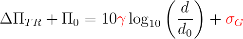
Where Π TR is the power difference between the transmitted and received signals. We are solving for the variables in red (path loss exponent and gaussian noise power) so that we can determine roughly where they fall for given scenarios. First, we need to determine the Π 0 for the given reference distance. I chose 1 meter here.
- Experimental Procedure for Finding γ and σG -
- Establish reference distance and power reading (I chose 1m)
- Calculate ΔΠ TR for multiple distances (at least 2, but more are receommended)
- Derive values for γ and σG
- Repeat for multiple scenarios (inside, outside, closed doors, etc.)
At this point in your experiment there should be a rough equation for distance for a given RSSI. Below are some statistical tools that can be used for better approximating physical degradation of the radio signal. These will give us a better estimate of the distance between the transmitter and receiver. See the list below for calculating a more accurate displacement from RSSI:
- Statistical Tools for Improving Distance Calculation from RSSI -
- Use Kalman Filter (average previous samples and weight them)
- Use time difference between received signals to improve γ approximation
- Incorporate standard deviation and RSSI sign change to determine if device is moving toward or away from receiver
Results
First, I chose a reference distance of 1 meter, which resulted in an RSSI of -48 dB. Therefore, d0 = 1, Π0 = -48, and our units are meters and decibels. I am using a transmitted power of 0 dB so that the value for ΔΠTR can be simplified to −ΠR. If you are using another power level (typically -23 dB, -6 dB, +6 dB), then the difference in power should be accounted for. This produces the final and simplified implicit equation that we will use to solve for path loss exponent and gaussian noise power:

| Distance [m] | RSSI [dB] | t [s] | Stand. Dev. [dB] | Size of k-filter [samples] | Sample Period [s] | Environment Notes |
|---|---|---|---|---|---|---|
| 0.5 | -45 | 0.49 | 8 | 15 | 30 | N/A |
| 1 | -48 | 0.48 | 7.4 | 15 | 30 | N/A |
| 2 | -59 | 0.6 | 7 | 15 | 30 | Against wall |
| 3 | -67 | 0.57 | 8.4 | 15 | 30 | Few nearby objects |
From the table of values above and a fit of the noise and path loss exponent, I found values of γ = 3, σG = 6.7 for a somewhat occupied apartment with a narrow area. These values are for an open path, without any blockage due to walls or objects (for the most part).
| Distance [m] | RSSI [dB] | t [s] | Stand. Dev. [dB] | Size of k-filter [samples] | Sample Period [s] | Environment Notes |
|---|---|---|---|---|---|---|
| 0.6 | -50.5 | 0.57 | 7.7 | 15 | 30 | 1 wall |
| 1 | -57 | 0.76 | 9.5 | 15 | 30 | 1 wall |
| 2 | -71 | 0.64 | 10.7 | 15 | 30 | 1 wall |
| 3 | -76 | 0.73 | 7 | 15 | 30 | 1 wall |
Table 2 values indicate roughly the same path loss exponent, γ = 3.6, but a larger gaussian noise of σG = 10.8.

Figure 2: This figure shows a complete route for a transceiver. The transceiver starts just a few inches away from the receiver, then moves to roughly 5.5 meters, then returns to its starting position. There is some noise due to obstacles which creates the jagged start, however, the return trip proves to be smoother. Also note the statistical variables that indicate changes in standard deviation (transceiver moving), changes in time between received signals (further away/more obstacles in path), and average changes in the RSSI (transceiver moving away or toward receiver).

RSSI Plot with Statistics
Figure 3: This plot demonstrates the complex nature of RSSI plots. This particular plot consists of 30 seconds of RSSI data averaged every 15 samples. The transmitter was placed about 3 meters away from the receiver and was in open air. Notice the sudden decline (despite there being no change in surrounding). This type of behavior makes analysis of RSSI difficult.
- Signal Processing Results -
For this section, attention was focused on smoothing data and producing the most stable results. Below is a series of figures that used a set route to approximate and test the accuracy of the distance approximation introduced above. Overall, the results were as expected. There is an omnipresent variability between data points, regardless of whether the sensor is moving. This means that at any given moment, the distance calculation can be floating around the true value with deviations as large as a few meters. Figure 4 below shows two runs of the same route, but with a large pause between outgoing and return trips in the second plot (to the right or below, depending on your browser). This indicates that the algorithm is repeatable, of course with large amounts of noise.
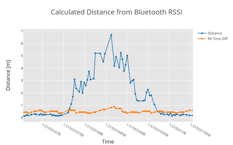

Figure 4: Example of real-time distance approximations for an HM-10 module going from 0.15 meters to approximately 7.3 meters and returning to 0.15 meters. You can see there's quite a bit of noise for both plots and that the return trip does not necessarily mimic the behavior of the outgoing trip. The calculations above used 3 and 7 for the path loss exponent and the average noise, respectively. The data was also acquired in a somewhat open room with a few obstacles. For the Kalman filter, 5 points were used, and the new point was weighted 30%, which meant that 70% of the signal depended on the previous points. This helped reduce the noise and variability in the results. Both figures represent the same route, where the second figure (on the right, or below depending on your browser) has a long gap between outgoing and return trips.

Figure 5: Repeated trips showing the range of accuracy over several back-to-back iterations of the same route. The starting point for the route was roughly 0.15 m and the farthest point was about 7.3 m. The accuracy at any given time was between 50%-300%. This means that high accuracy for distance calculations using RSSI is not attainable in this simple case.
Conclusions
In these two articles on distance approximation using RSSI, I was able to show with a decent degree of accuracy that Bluetooth modules such as the HM-10, along with the Raspberry Pi, are capable of creating a network of reliable iBeacons. I tested an HM-10 several different ways and presented methods for creating a series of sensors that can approximate displacement between receiver and transmitter. And although the results were noisy, I was still capable of resolving three simultaneous trips from the receiver to approximately 7 meters away very good agreement between the three tests. This concluded that, with some advanced signal processing and utilization of Kalman filtering and derivative analysis, a system of wireless, inexpensive, Bluetooth-powered iBeacons (HM-10 modules) can be used to approximate their relative distance to another device within a margin of error that decreases with distance. This could be significant for industries interested in proximity sensing, asset tracking, proximity authorization, and even indoor navigation. Bluetooth Low Energy is a powerful tool, and beacon technology is becoming more and more popular because of its low cost, versatile, and reliable advantages. I hope these brief entries inspire someone to create something unique and innovative beyond my own imagination.
See More in Internet of Things: