Loudspeaker Analysis and Experiments: Part I

Thiele-Small Parameters and Background
Parts List for Experiments
Measuring the DC Coil Resistance
Wiring for Impedance Measurement
Identifying the Resonance Region Using a Full-Spectrum Frequency Sweep
Impedance Magnitude and Phase Relation to Resonance
Conclusion and Continuation
A modern loudspeaker is a crossover technology comprised of electrical and mechanical components. And while this design helps humans enjoy the analog world using digitization, it also creates a complex problem that encompasses the fields of fluid dynamics and electrical engineering. In order to demystify the loudspeaker, two engineers: Neville Thiele and Richard H. Small derived relationships between the physical parameters of a loudspeaker and its acoustic performance. These parameters, called the Thiele-Small Parameters, are still used today to design audio systems and remain a cornerstone for quantifying the performance of such a system [read more about Thiele-Small Parameters here and here, and design aspects here and here].
In this tutorial, a loudspeaker will be analyzed by calculating the Thiele-Small parameters from impedance measurements using an inexpensive USB data acquisition system (minimum sampling rate of 44.1 kHz). The methods used in this project will educate the user on multiple engineering topics ranging from: data acquisition, electronics, acoustics, signal processing, and computer programming.

1. Magnet, 2. Voice Coil (Inductive Coil), 3. Suspension, 4. Diaphragm
A few crutial Thiele-Small pararmeters are cited below based on the Thiele and Small papers:
The parameters above give information about the speaker’s performance and limitations, which define some physical characteristics of the loudspeaker. These characteristics are difficult to quantify once the loudspeaker is assembled, so we are forced to approximate the following physical characteristics using experiments:
A few notes on the definitions above: r represents a parameter calculated at the loudspeaker’s resonance frequency. Additionally, e represents a parameter in the electrical domain; m represents a parameter in the mechanical domain, and a represents the acoustic domain. From this point onward, I will use each parameter to define another parameter using specific equation derived by Thiele and Small.
This is a fairly involved experiment in that it requires the following core parts: a computer, a USB acquisition device (at least 44.1 kHz sampling rate), a loudspeaker driver, and small calibration weights. These components will allow us to fully characterize the loudspeaker using the Thiele-Small parameters. Below is the full parts list used in my method of calculating the parameters:
Boss Audio 80 Watt Loudspeaker - $10.79 [Amazon]
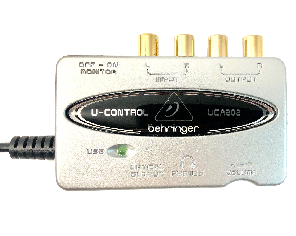
Behringer UCA202 USB Audio Interface - $29.99 [Amazon]
Calibration Weights - $6.99 [Amazon]
Audio Amplifier 15 Watt - $8.99 [Amazon]
Speaker Wire - $8.49 [Amazon]
Multimeter with AC Voltmeter - $37.97 [Amazon]
Alligator Clips - $6.39 [Amazon]
Jumper Wires - $6.49 [Amazon]
Resistor Kit - $7.99 [Amazon]
Breadboard - $7.99 [Amazon]
3.5 mm cable - $5.10 [Amazon]

Boss Audio Full Range 80W Driver
The first step in the process is to measure the speaker’s electrical resistance, which should always be less than the nominal resistance. Start by measuring the resistance of the leads on your multimeter, then subtract that from the resistance measured across the terminals of the speaker. I measured the resistance to be 3.3 Ohms:
The wiring for this experiment is somewhat involved, however, the root of the wiring method is based on a voltage divider with the speaker acting as the second resistor. The full diagram is shown below:
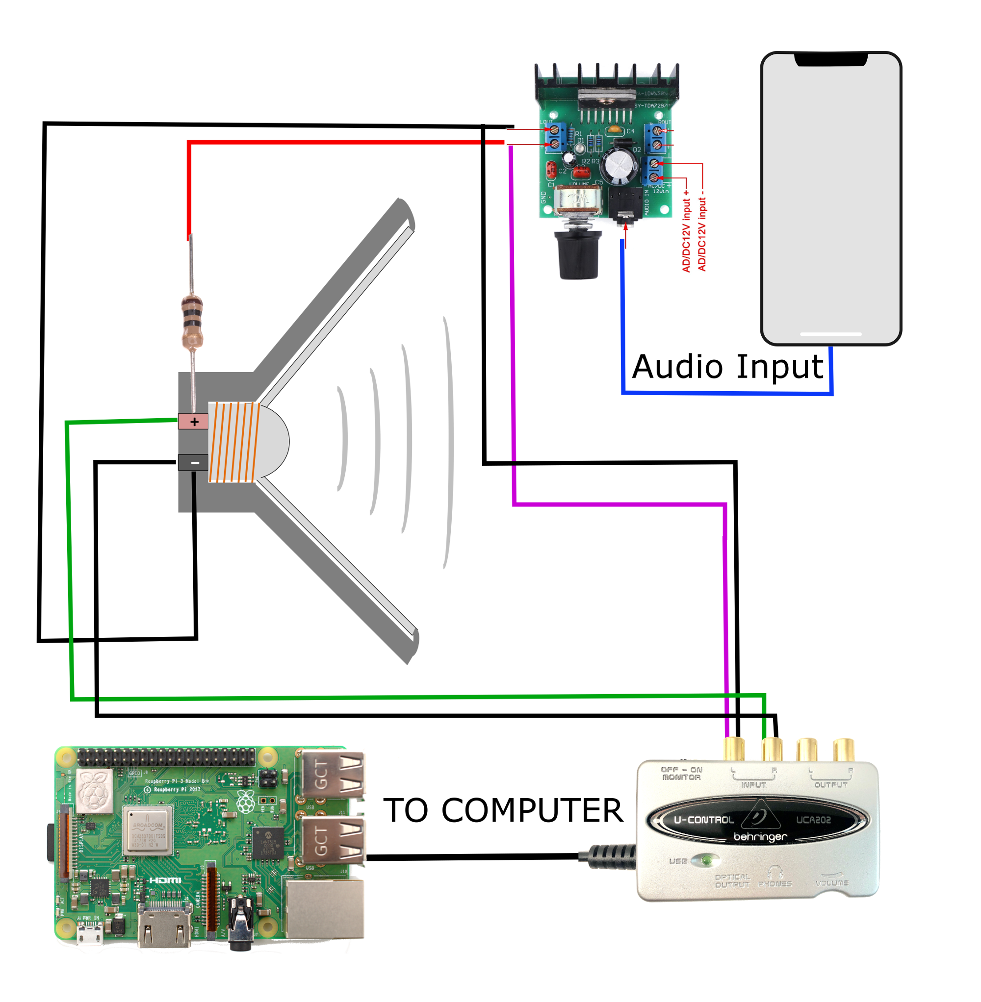
The process flow for the wiring above is as follows:
A smartphone app called ‘Audio Function Generator’ is used to generate a sine wave sweep or constant frequency into the amplifier’s 3.5 mm input
The amplified signal is wired across the voltage divider
The voltage across the amplified signal is inputted into the Behringer USB acquisition device
The voltage across the loudspeaker terminals is inputted into the Behringer USB acquisition device
The USB stereo input is read by Python on a computer (Raspberry Pi in my case)
Using the wiring method above, we will be able to approximate the resonance frequency of the driver where the impedance is maximum. We will also be able to find parameters relating to the electrical and mechanical properties of the driver.
We’ll be using the Behringer UCA202 USB audio interface to sample voltage readings at 44.1 kHz on a Raspberry Pi. The general setup for finding the resonance frequency starts by wiring the loudspeaker in series with a resistor to measure voltage across the speaker. And since the voltage varies when we excite the speaker using a sinusoidal function, we need to approximate the impedance across the loudspeaker. The voltage divider equation can be rewritten specifically for our scenario:
An impedance plot of the loudspeaker that I used is shown below for a frequency sweep from 20 Hz - 20,000 Hz. I sampled the impedance over 180 seconds. It was done in three pieces and then stitched together. I used the ranges of 20 Hz - 120 Hz, 120 Hz - 2,000 Hz, and 2,000 Hz - 20,000 Hz. This was done to avoid diminishing the peak and the transition zone between high and low frequencies. I used a sampling period of 1 second, which resulted in a frequency resolution of 1 Hz.

Impedance Plot Identifying Resonance Region
There are also a few extraneous peaks that likely represent some sort of noise in the input signal. The noise is likely due to the sampling interval and how the smartphone app handles the sweep. Also - the user may notice an increase in the impedance as the frequency increases toward infinity. This is often cited as an artifact of the speaker's inductance, which can act as a frequency filter (hence the increase in impedance with frequency).
The important thing to remember is that we have identified the resonance region of the loudspeaker, which we will further explore in the next section when we discuss phase behavior and approximating the amplitude of the impedance at resonance.
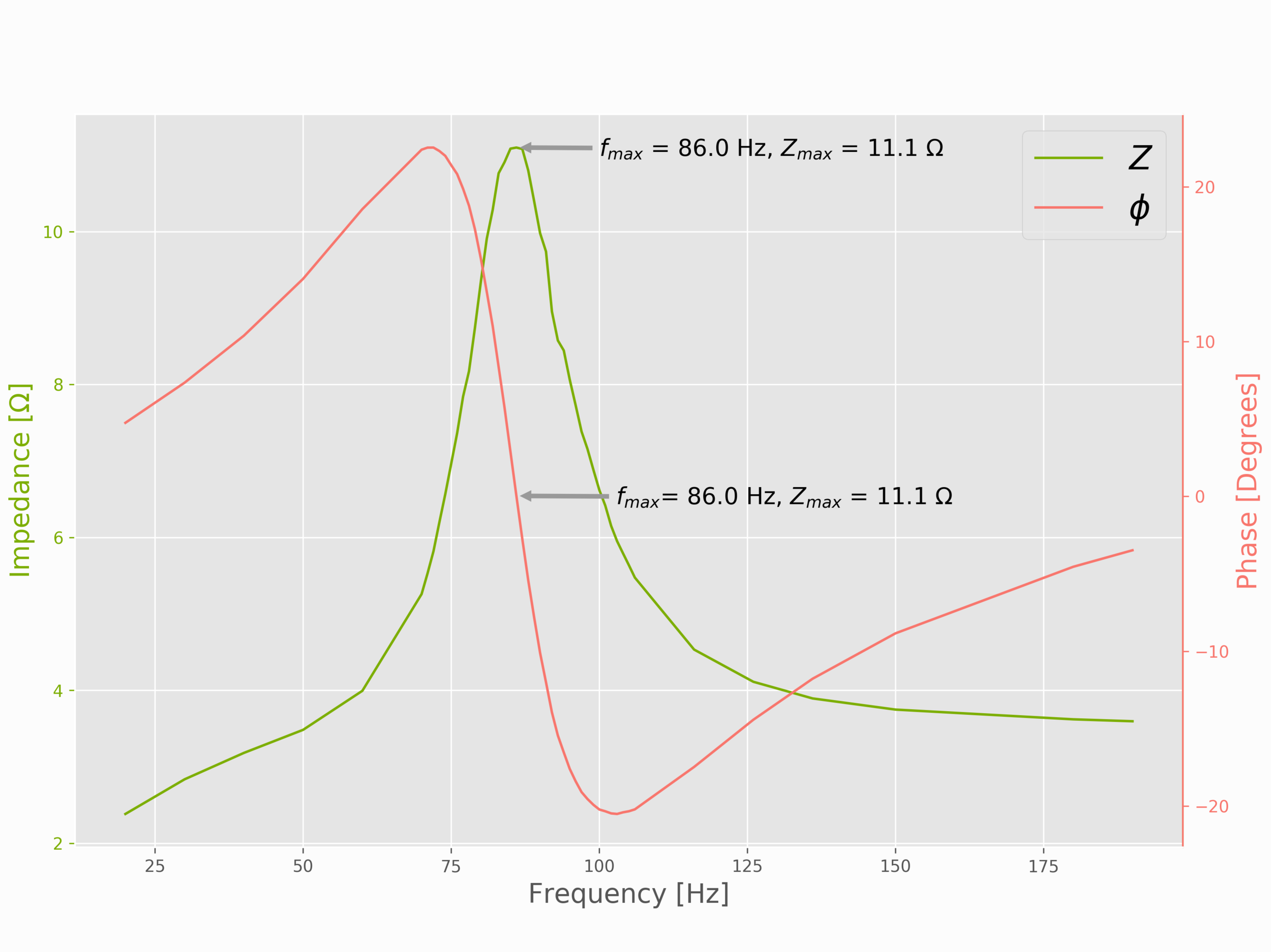
There are multiple ways of identifying the actual resonance frequency of a loudspeaker. Many manufacturers will put the impedance response curve on their datasheet, and fewer will include the phase measurement, which is often correlated to the derivative of the impedance. This means that if we plot both the impedance response and the phase, we should see a phase zero-crossing around the resonance frequency.
The response curves for phase and impedance can be seen below calculated for the loudspeaker used in this project (44.1kHz, 10 sec recording, 20 Hz - 220 Hz sweep):

The full code to replicate the figures above is also given below
import pyaudio
import numpy as np
import matplotlib.pyplot as plt

plt.style.use('ggplot')

def fft_calc(data_vec):
    fft_data_raw = (np.fft.fft(data_vec))
    fft_data = (fft_data_raw[0:int(np.floor(len(data_vec)/2))])/len(data_vec)
    fft_data[1:] = 2*fft_data[1:]
    return fft_data

form_1 = pyaudio.paInt16 # 16-bit resolution
chans = 2 # 1 channel
samp_rate = 44100 # 44.1kHz sampling rate
record_secs = 10 # seconds to record
dev_index = 2 # device index found by p.get_device_info_by_index(ii)
chunk = 44100*record_secs # 2^12 samples for buffer
R_1 = 9.8 # measured resistance from voltage divider resistor
R_dc = 3.3 # measured dc resistance of loudspeaker

freq_sweep_range = (40.0,200.0) # range of frequencies in sweep (plus or minus a few to avoid noise at the ends)

audio = pyaudio.PyAudio() # create pyaudio instantiation

# create pyaudio stream
stream = audio.open(format = form_1,rate = samp_rate,channels = chans, \
                    input_device_index = dev_index,input = True, \
                    frames_per_buffer=chunk)

stream.stop_stream() # pause stream so that user can control the recording
input("Click to Record")

data,chan0_raw,chan1_raw = [],[],[]

# loop through stream and append audio chunks to frame array
stream.start_stream() # start recording
for ii in range(0,int((samp_rate/chunk)*record_secs)):
    data.append(np.fromstring(stream.read(chunk),dtype=np.int16))

# stop, close stream, and terminate pyaudio instantiation
stream.stop_stream()
stream.close()
audio.terminate()

print("finished recording\n------------------")

# loop through recorded data to extract each channel
for qq in range(0,(np.shape(data))[0]):
    curr_dat = data[qq]
    chan0_raw.append(curr_dat[::2])
    chan1_raw.append((curr_dat[1:])[::2])

# conversion from bits
chan0_raw = np.divide(chan0_raw,(2.0**15)-1.0)
chan1_raw = np.divide(chan1_raw,(2.0**15)-1.0)

# Calculating FFTs and phases
spec_array_0_noise,spec_array_1_noise,phase_array,Z_array = [],[],[],[]
for mm in range(0,(np.shape(chan0_raw))[0]):
    Z_0 = ((fft_calc(chan0_raw[mm])))
    Z_1 = ((fft_calc(chan1_raw[mm])))

    phase_array.append(np.subtract(np.angle(Z_0,deg=True),
                                   np.angle(Z_1,deg=True)))

    spec_array_0_noise.append(((np.abs(Z_0[1:]))))
    spec_array_1_noise.append(((np.abs(Z_1[1:]))))

# frequency values for FFT
f_vec = samp_rate*np.arange(chunk/2)/chunk # frequency vector
plot_freq = f_vec[1:] # avoiding f = 0 for logarithmic plotting

# calculating Z
Z_mean = np.divide(R_1*np.nanmean(spec_array_0_noise,0),
           np.subtract(np.nanmean(spec_array_1_noise,0),np.nanmean(spec_array_0_noise,0)))

# setting minimum frequency locations based on frequency sweep
f_min_loc = np.argmin(np.abs(plot_freq-freq_sweep_range[0]))
f_max_loc = np.argmin(np.abs(plot_freq-freq_sweep_range[1]))
max_f_loc = np.argmax(Z_mean[f_min_loc:f_max_loc])+f_min_loc
f_max = plot_freq[max_f_loc]

# print out impedance found from phase zero-crossing
print('Resonance at Z-based Maximum:')
print('f = {0:2.1f}, Z = {1:2.1f}'.format(f_max,np.max(Z_mean[f_min_loc:f_max_loc])))
print('------------------')

# smoothing out the phase data by averaging large spikes

smooth_width = 10 # width of smoothing window for phase
phase_trimmed = (phase_array[0])[f_min_loc:f_max_loc]
phase_diff = np.append(0,np.diff(phase_trimmed))
for yy in range(smooth_width-1,len(phase_diff)-smooth_width):
    for mm in range(0,smooth_width):
        if np.abs(phase_diff[yy]) > 100.0:
            phase_trimmed[yy] = (phase_trimmed[yy-mm]+phase_trimmed[yy+mm])/2.0
            phase_diff[yy] = (phase_diff[yy-mm]+phase_diff[yy+mm])/2.0
        if np.abs(phase_diff[yy]) > 100.0:
            continue
        else:
            break
    if np.abs(phase_diff[yy]) > 100.0:
        phase_trimmed[yy] = np.nan

##### plotting algorithms for impedance and phase ####

fig,ax = plt.subplots()
fig.set_size_inches(12,8)

# Logarithm plots in x-axis
p1, = ax.semilogx(plot_freq[f_min_loc:f_max_loc],Z_mean[f_min_loc:f_max_loc],label='$Z$',color='#7CAE00')
ax2 = ax.twinx() # mirror axis for phase
p2, = ax2.semilogx(plot_freq[f_min_loc:f_max_loc],phase_trimmed,label='$\phi$',color='#F8766D')

# plot formatting
subplot_vec = [p1,p2]
ax2.legend(subplot_vec,[l.get_label() for l in subplot_vec],fontsize=20)
ax.yaxis.label.set_color(p1.get_color())
ax2.yaxis.label.set_color(p2.get_color())
ax.set_ylabel('Impedance [$\Omega$]',fontsize=16)
ax2.set_ylabel('Phase [Degrees]',fontsize=16)
ax2.grid(False)
ax.spines["right"].set_edgecolor(p1.get_color())
ax2.spines["right"].set_edgecolor(p2.get_color())
ax.tick_params(axis='y', colors=p1.get_color())
ax2.tick_params(axis='y', colors=p2.get_color())
ax.set_xlabel('Frequency [Hz]',fontsize=16)

peak_width = 70.0 # approx width of peak in Hz
ax.set_xlim([f_max-(peak_width/2.0),f_max+(peak_width/2.0)])
ax.set_ylim([np.min(Z_mean[f_min_loc:f_max_loc]),np.max(Z_mean[f_min_loc:f_max_loc])+0.5])
ax2.set_xlim([f_max-(peak_width/2.0),f_max+(peak_width/2.0)])
ax2.set_ylim([-45,45])
ax.set_xticks([],minor=True)
ax2.set_xticks(np.arange(f_max-(peak_width/2.0),f_max+(peak_width/2.0),10))
ax2.set_xticklabels(['{0:2.0f}'.format(ii) for ii in np.arange(f_max-(peak_width/2.0),f_max+(peak_width/2.0),10)])

# locating phase and Z maximums to annotate the figure
Z_max_text = ' = {0:2.1f} $\Omega$'.format(np.max(Z_mean[f_min_loc:f_max_loc]))
f_max_text = ' = {0:2.1f} Hz'.format(plot_freq[np.argmax(Z_mean[f_min_loc:f_max_loc])+f_min_loc])
ax.annotate('$f_{max}$'+f_max_text+', $Z_{max}$'+Z_max_text,xy=(plot_freq[np.argmax(Z_mean[f_min_loc:f_max_loc])+f_min_loc],
                                                                np.max(Z_mean[f_min_loc:f_max_loc])),\
            xycoords='data',xytext=(-300,-50),size=14,textcoords='offset points',
                   arrowprops=dict(arrowstyle='simple',
                                   fc='0.6',ec='none'))
# from phase
phase_f_min = np.argmin(np.abs(np.subtract(f_max-(peak_width/2.0),plot_freq)))
phase_f_max = np.argmin(np.abs(np.subtract(f_max+(peak_width/2.0),plot_freq)))
phase_min_loc = np.argmin(np.abs(phase_array[0][phase_f_min:phase_f_max]))+phase_f_min

Z_max_text_phase = ' = {0:2.1f} $\Omega$'.format(Z_mean[phase_min_loc])
f_max_text_phase = ' = {0:2.1f} Hz'.format(plot_freq[phase_min_loc])
ax2.annotate('$\phi_{min}$'+' ={0:2.1f}$^\circ$'.format(np.abs(phase_array[0][phase_min_loc]))+', $f_{max}$ = '+f_max_text_phase+\
             '\n$Z_{max}$'+Z_max_text_phase,
             xy=(plot_freq[phase_min_loc],phase_array[0][phase_min_loc]),\
            xycoords='data',xytext=(-120,-150),size=14,textcoords='offset points',arrowprops=dict(arrowstyle='simple',
                                   fc='0.6',ec='none'))
# print out impedance found from phase zero-crossing
print('Resonance at Phase Zero-Crossing:')
print('f = {0:2.1f}, Z = {1:2.1f}'.format(plot_freq[phase_min_loc],Z_mean[phase_min_loc]))

# uncomment to save plot
##plt.savefig('Z_sweep_with_phase.png',dpi=300,facecolor=[252/255,252/255,252/255])

plt.show()
The code above and all the codes for this project can be found on the project’s GitHub page:
Therefore, for the case of our loudspeaker - we can say that its resonance frequency is about 86 Hz. And by using the actual RMS values of steady frequency inputs, I have another plot that shows just how close this is to the likely resonance:
Plot of impedance and phase around resonance
This method is done by hand, not using an FFT. We can still see similar behavior using this method, indicating that the FFT method is accurate (and time-saving).
The manual method shown directly above can be used to approximate the resonance, however, I will use the quicker and nearly as accurate FFT method. And in the next entry, we will be doing multiple measurements of resonance at different mass loadings - so the manual method would really time quite a bit of time.
In this first entry into the loudspeaker analysis series, I discussed the Thiele-Small parameters and the notion of impedance and resonance. The complex nature of loudspeakers makes this series an educational and diverse topic in engineering. I explored how to find the resonance frequency of a speaker driver and how to use both phase and magnitude to approximate the frequency of the resonance and the magnitude of the impedance at resonance. Both of these values will become instrumental in characterizing loudspeakers and audio systems for use in real-world applications.
In the next entry, I discuss how to find the remaining mechanical and electrical properties of a loudspeaker and the applications that they open up in terms of design in acoustic environments.

See More in Acoustics and Engineering: