Recording Stereo Audio on a Raspberry Pi
“As an Amazon Associates Program member, clicking on links may result in Maker Portal receiving a small commission that helps support future projects.”
Raspberry Pi boards are capable of recording stereo audio using an interface called the inter-IC sound (I2S or I2S) bus. The I2S standard uses three wires to record data, keep track of timing (clock), and determine whether an input/output is in the left channel or right channel [read more on I2S here and here]. First, the Raspberry Pi (RPi) needs to be prepped for I2S communication by creating/enabling an audio port in the RPi OS system. This audio port will then be used to communicate with MEMS microphones and consequently record stereo audio (one left channel, one right channel). Python iS then used to record the 2-channel audio via the pyaudio Python audio library. Finally, the audio data will be visualized and analyzed in Python with simple digital signal processing methods that include Fast Fourier Transforms (FFTs), noise subtraction, and frequency spectrum peak detection.
I2S Tutorial from Adafruit:
https://learn.adafruit.com/adafruit-i2s-mems-microphone-breakout/raspberry-pi-wiring-test

Step 1. Load the RPi OS onto the SD Card
Once the Raspberry Pi OS is loaded onto the SD card, insert the card into the RPi board. A Raspberry Pi 4 Model B board is used going forward.
Step 2: Update and Upgrade the RPi
pi@raspberrypi:~ $ sudo apt-get -y update
pi@raspberrypi:~ $ sudo apt-get -y upgrade
pi@raspberrypi:~ $ sudo reboot
Step 3: Install Python 3 Libraries and I2S Module
We start by installing Python3 and pip:
pi@raspberrypi:~ $ sudo apt install python3-pip
Next, it is good to install the Python Integrated Development Learning Environment (IDLE), where we can write scripts and visualize data a bit easier:
pi@raspberrypi:~ $ sudo apt-get install idle3
pi@raspberrypi:~ $ sudo pip3 install --upgrade adafruit-python-shell
pi@raspberrypi:~ $ sudo wget https://raw.githubusercontent.com/adafruit/Raspberry-Pi-Installer-Scripts/master/i2smic.py
Assuming the above did not result in any errors, we can run the .py file that installs the i2smic capability onto the RPi:
pi@raspberrypi:~ $ sudo python3 i2smic.py
The following prompt will ask the user whether they want the I2S input to be loaded at boot. ‘y’ should be inputted, unless the user has a preference to keep the boot minimal (not recommended for heavy audio use).

After agreeing to load at boot, the install will take several minutes (depending on internet speed). Once the install completes, the user will again be prompted to reboot. Reboot and then continue with the next step.
Step 4: Install pyaudio libraries for Python Analyses
pi@raspberrypi:~ $ sudo apt-get install libportaudio0 libportaudio2 libportaudiocpp0 portaudio19-dev
pi@raspberrypi:~ $ sudo pip3 install pyaudio matplotlib scipy
################################
# Checking I2S Input in Python
################################
#
import pyaudio

audio = pyaudio.PyAudio() # start pyaudio
for ii in range(0,audio.get_device_count()):
    # print out device info
    print(audio.get_device_info_by_index(ii))
The following should be outputted to the Python shell:

'snd_rpi_i2s_card' is our I2S Module that Communicates with our MEMS Microphones
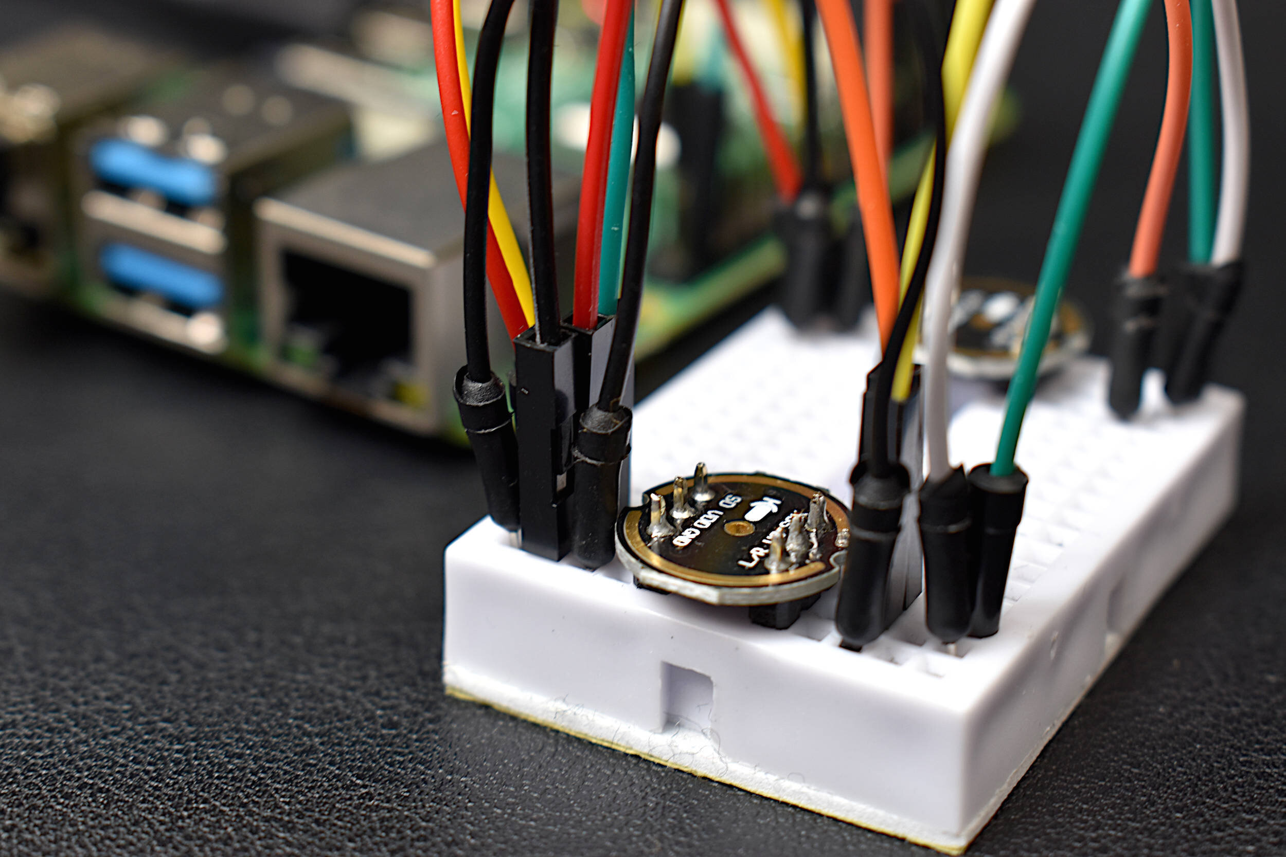
1x Raspberry Pi 4B Computer (4GB RAM) - $57.99 [Board Only on: Amazon], $99.99 [Kit on Amazon], $55.00 [2GB from Our Store]
2x INMP441 MEMS Microphones - $10.00 [Our Store]
1x Mini Breadboard - $3.00 [Our Store]
7x Male-to-Male Jumper Wires - $1.05 [Our Store]
5x Male-to-Female Jumper Wires - $0.75 [Our Store]
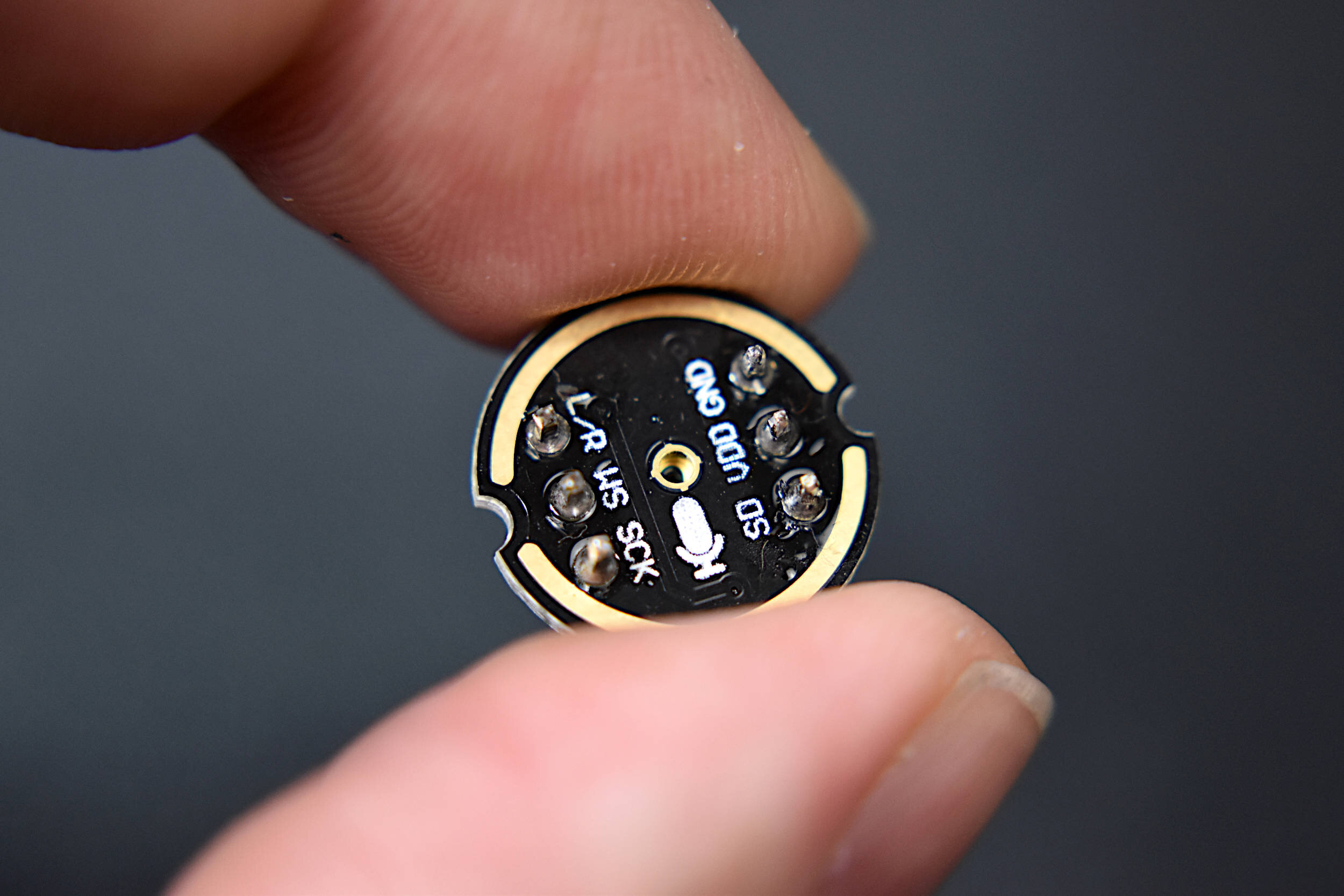
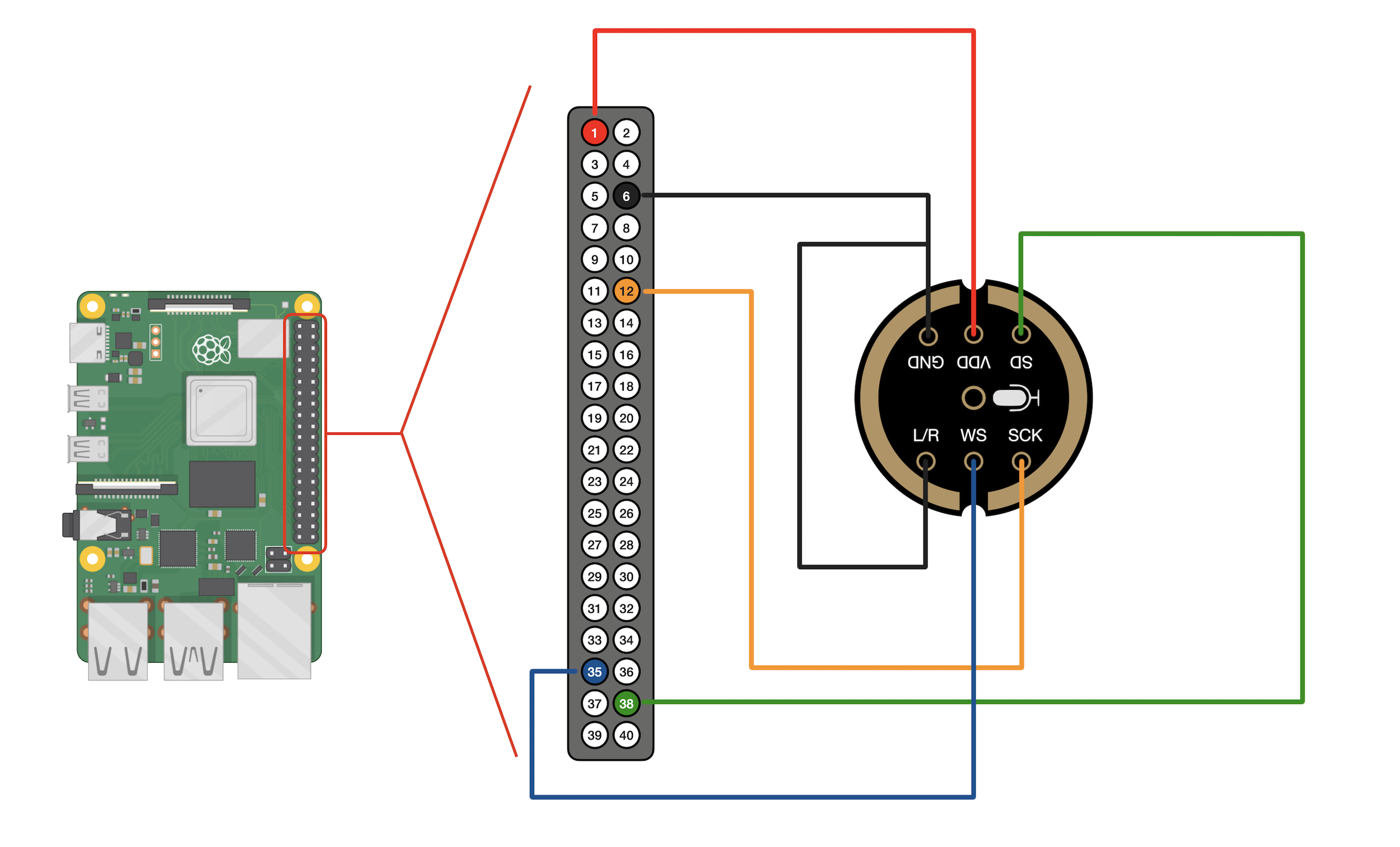
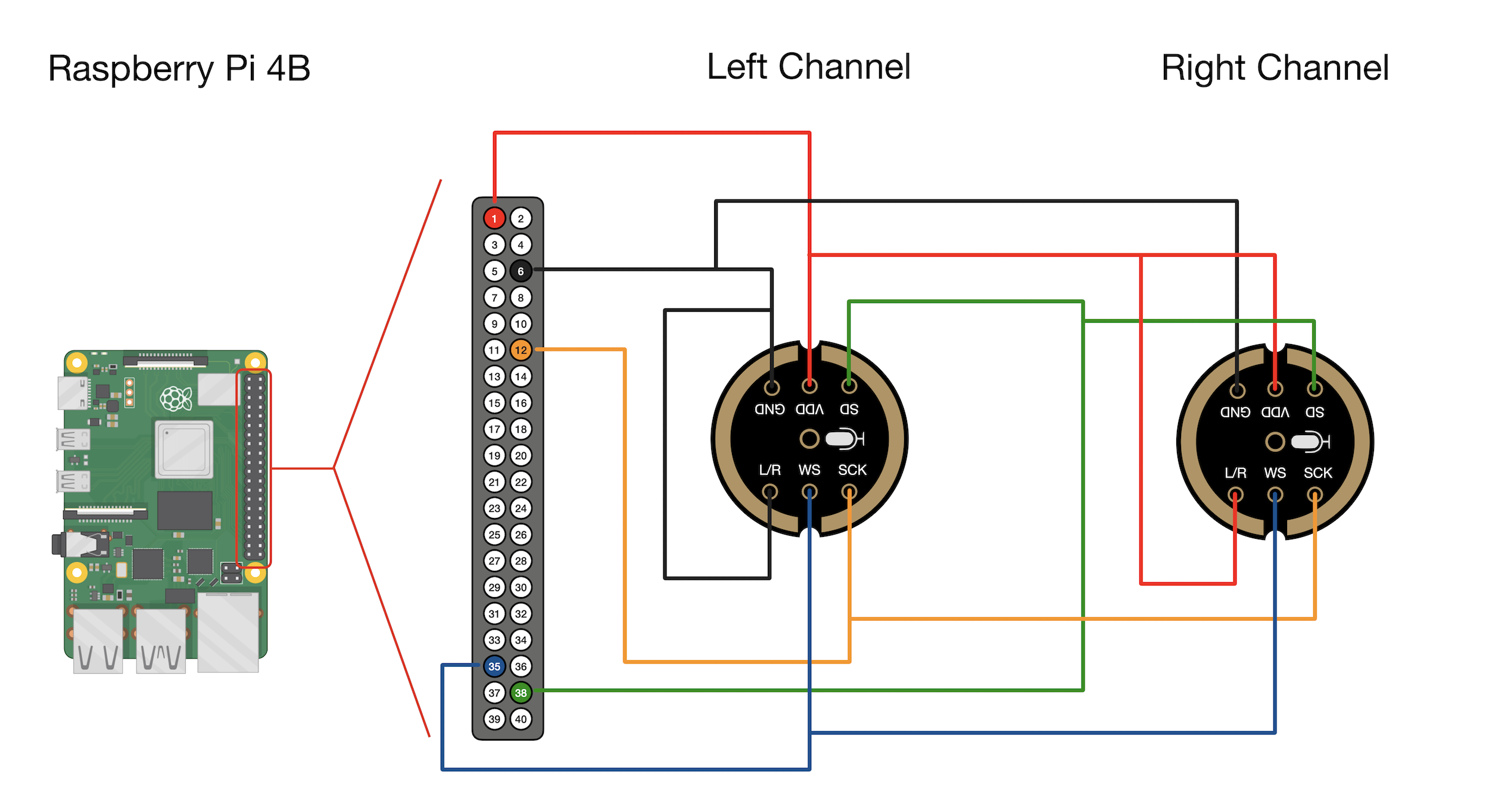
The wiring diagram between the Raspberry Pi computer and the INMP441 MEMS Microphone is given below:
Mono Microphone Input
Stereo Microphone Input
| Raspberry Pi | INMP441 (Left) | INMP441 (Right) |
|---|---|---|
| 3V3 | VDD | VDD |
| Ground | GND | GND |
| GPIO 18 (PCM_CLK) | SCK | SCK |
| GPIO 19 (PCM_FS) | WS | WS |
| GPIO 20 (PCM_DIN) | SD | SD |
| Ground | L/R | |
| 3V3 | L/R |
Record 1 second of background noise (at 44.1kHz sample rate)
Record 5 seconds of data
Save the recorded audio as a .wav file under a folder called ‘data’ with the filename corresponding to the current date/time
Remove the background noise from the 5 seconds data
Select the peak frequency of the frequency response (computed with the Numpy FFT)
Plot the time series and frequency response of the 5 second recording
##############################################
# INMP441 MEMS Microphone + I2S Module
##############################################
#
# -- Frequency analysis with FFTs and saving
# -- .wav files of MEMS mic recording
#
# --------------------------------------------
# -- by Josh Hrisko, Maker Portal LLC
# --------------------------------------------
#
##############################################
#
import pyaudio
import matplotlib.pyplot as plt
import numpy as np
import time,wave,datetime,os,csv

##############################################
# function for FFT
##############################################
#
def fft_calc(data_vec):
    data_vec = data_vec*np.hanning(len(data_vec)) # hanning window
    N_fft = len(data_vec) # length of fft
    freq_vec = (float(samp_rate)*np.arange(0,int(N_fft/2)))/N_fft # fft frequency vector
    fft_data_raw = np.abs(np.fft.fft(data_vec)) # calculate FFT
    fft_data = fft_data_raw[0:int(N_fft/2)]/float(N_fft) # FFT amplitude scaling
    fft_data[1:] = 2.0*fft_data[1:] # single-sided FFT amplitude doubling
    return freq_vec,fft_data
#
##############################################
# function for setting up pyserial
##############################################
#
def pyserial_start():
    audio = pyaudio.PyAudio() # create pyaudio instantiation
    ##############################
    ### create pyaudio stream  ###
    # -- streaming can be broken down as follows:
    # -- -- format             = bit depth of audio recording (16-bit is standard)
    # -- -- rate               = Sample Rate (44.1kHz, 48kHz, 96kHz)
    # -- -- channels           = channels to read (1-2, typically)
    # -- -- input_device_index = index of sound device
    # -- -- input              = True (let pyaudio know you want input)
    # -- -- frmaes_per_buffer  = chunk to grab and keep in buffer before reading
    ##############################
    stream = audio.open(format = pyaudio_format,rate = samp_rate,channels = chans, \
                        input_device_index = dev_index,input = True, \
                        frames_per_buffer=CHUNK)
    stream.stop_stream() # stop stream to prevent overload
    return stream,audio

def pyserial_end():
    stream.close() # close the stream
    audio.terminate() # close the pyaudio connection
#
##############################################
# function for plotting data
##############################################
#
def plotter(plt_1=0,plt_2=0):
    plt.style.use('ggplot')
    plt.rcParams.update({'font.size':16})
    ##########################################
    # ---- time series and full-period FFT
    if plt_1:
        fig,axs = plt.subplots(2,1,figsize=(12,8)) # create figure
        ax = axs[0] # top axis: time series
        ax.plot(t_vec,data,label='Time Series') # time data
        ax.set_xlabel('Time [s]') # x-axis in time
        ax.set_ylabel('Amplitude') # y-axis amplitude
        ax.legend(loc='upper left')

        ax2 = axs[1] # bottom axis: frequency domain
        ax2.plot(freq_vec,fft_data,label='Frequency Spectrum')
        ax2.set_xscale('log') # log-scale for better visualization
        ax2.set_yscale('log') # log-scale for better visualization
        ax2.set_xlabel('Frequency [Hz]')# frequency label
        ax2.set_ylabel('Amplitude') # amplitude label
        ax2.legend(loc='upper left')

        # peak finder labeling on the FFT plot
        max_indx = np.argmax(fft_data) # FFT peak index
        ax2.annotate(r'$f_{max}$'+' = {0:2.1f}Hz'.format(freq_vec[max_indx]),
                     xy=(freq_vec[max_indx],fft_data[max_indx]),
                     xytext=(2.0*freq_vec[max_indx],
                             (fft_data[max_indx]+np.mean(fft_data))/2.0),
                     arrowprops=dict(facecolor='black',shrink=0.1)) # peak label

    ##########################################
    # ---- spectrogram (FFT vs time)
    if plt_2:
        fig2,ax3 = plt.subplots(figsize=(12,8)) # second figure
        t_spec = np.reshape(np.repeat(t_spectrogram,np.shape(freq_array)[1]),np.shape(freq_array))
        y_plot = fft_array # data array
        spect = ax3.pcolormesh(t_spec,freq_array,y_plot,shading='nearest') # frequency vs. time/amplitude
        ax3.set_ylim([20.0,20000.0])
        ax3.set_yscale('log') # logarithmic scale in freq.
        cbar = fig2.colorbar(spect) # add colorbar
        cbar.ax.set_ylabel('Amplitude',fontsize=16) # amplitude label

    fig.subplots_adjust(hspace=0.3)
    fig.savefig('I2S_time_series_fft_plot.png',dpi=300,
                bbox_inches='tight')
    plt.show() # show plot
#
##############################################
# function for grabbing data from buffer
##############################################
#
def data_grabber(rec_len):
    stream.start_stream() # start data stream
    stream.read(CHUNK,exception_on_overflow=False) # flush port first
    t_0 = datetime.datetime.now() # get datetime of recording start
    print('Recording Started.')
    data,data_frames = [],[] # variables
    for frame in range(0,int((samp_rate*rec_len)/CHUNK)):
        # grab data frames from buffer
        stream_data = stream.read(CHUNK,exception_on_overflow=False)
        data_frames.append(stream_data) # append data
        data.append(np.frombuffer(stream_data,dtype=buffer_format))
    stream.stop_stream() # stop data stream
    print('Recording Stopped.')
    return data,data_frames,t_0
#
##############################################
# function for analyzing data
##############################################
#
def data_analyzer(chunks_ii):
    freq_array,fft_array = [],[]
    t_spectrogram = []
    data_array = []
    t_ii = 0.0
    for frame in chunks_ii:
        freq_ii,fft_ii = fft_calc(frame) # calculate fft for chunk
        freq_array.append(freq_ii) # append chunk freq data to larger array
        fft_array.append(fft_ii) # append chunk fft data to larger array
        t_vec_ii = np.arange(0,len(frame))/float(samp_rate) # time vector
        t_ii+=t_vec_ii[-1]
        t_spectrogram.append(t_ii) # time step for time v freq. plot
        data_array.extend(frame) # full data array
    t_vec = np.arange(0,len(data_array))/samp_rate # time vector for time series
    freq_vec,fft_vec = fft_calc(data_array) # fft of entire time series
    return t_vec,data_array,freq_vec,fft_vec,freq_array,fft_array,t_spectrogram
#
##############################################
# Save data as .wav file and .csv file
##############################################
#
def data_saver(t_0):
    data_folder = './data/' # folder where data will be saved locally
    if os.path.isdir(data_folder)==False:
        os.mkdir(data_folder) # create folder if it doesn't exist
    filename = datetime.datetime.strftime(t_0,
                                          '%Y_%m_%d_%H_%M_%S_pyaudio') # filename based on recording time
    wf = wave.open(data_folder+filename+'.wav','wb') # open .wav file for saving
    wf.setnchannels(chans) # set channels in .wav file
    wf.setsampwidth(audio.get_sample_size(pyaudio_format)) # set bit depth in .wav file
    wf.setframerate(samp_rate) # set sample rate in .wav file
    wf.writeframes(b''.join(data_frames)) # write frames in .wav file
    wf.close() # close .wav file
    return filename
#
##############################################
# Main Data Acquisition Procedure
##############################################
#
if __name__=="__main__":
    #
    ###########################
    # acquisition parameters
    ###########################
    #
    CHUNK          = 44100  # frames to keep in buffer between reads
    samp_rate      = 44100 # sample rate [Hz]
    pyaudio_format = pyaudio.paInt16 # 16-bit device
    buffer_format  = np.int16 # 16-bit for buffer
    chans          = 1 # only read 1 channel
    dev_index      = 0 # index of sound device
    #
    #############################
    # stream info and data saver
    #############################
    #
    stream,audio = pyserial_start() # start the pyaudio stream
    record_length =  5 # seconds to record
    input('Press Enter to Record Noise (Keep Quiet!)')
    noise_chunks,_,_ = data_grabber(CHUNK/samp_rate) # grab the data
    input('Press Enter to Record Data (Turn Freq. Generator On)')
    data_chunks,data_frames,t_0 = data_grabber(record_length) # grab the data
    data_saver(t_0) # save the data as a .wav file
    pyserial_end() # close the stream/pyaudio connection
    #
    ###########################
    # analysis section
    ###########################
    #
    _,_,_,fft_noise,_,_,_ = data_analyzer(noise_chunks) # analyze recording
    t_vec,data,freq_vec,fft_data,\
            freq_array,fft_array,t_spectrogram = data_analyzer(data_chunks) # analyze recording
    # below, we're subtracting noise
    fft_array = np.subtract(fft_array,fft_noise)
    freq_vec = freq_array[0]
    fft_data = np.mean(fft_array[1:,:],0)
    fft_data = fft_data+np.abs(np.min(fft_data))+1.0
    plotter(plt_1=1,plt_2=0) # select which data to plot
    #  ^(plt_1 is time/freq), ^(plt_2 is spectrogram)
The resulting output should look similar to the plot shown below:

A 3114Hz signal was inputted using a smartphone frequency generator placed a foot away from the INMP441 MEMS microphone. At this stage, with the frequency response matching the input frequency generated by the app - we are sure that the microphone is being read properly by the Raspberry Pi! It also may be noticeable that the amplitude is quite low on the mic response - we will address this as well as the adjustments to be made to the code in order to permit stereo recording.

##############################################
# STEREO INMP441 MEMS Microphone + I2S Module
##############################################
#
# -- Stereo frequency analysis with FFTs and
# -- saving .wav files of MEMS mic recording
#
# --------------------------------------------
# -- by Josh Hrisko, Maker Portal LLC
# --------------------------------------------
#
##############################################
#
import pyaudio
import matplotlib.pyplot as plt
import numpy as np
import time,wave,datetime,os,csv

##############################################
# function for FFT
##############################################
#
def fft_calc(data_vec):
    data_vec = data_vec*np.hanning(len(data_vec)) # hanning window
    N_fft = len(data_vec) # length of fft
    freq_vec = (float(samp_rate)*np.arange(0,int(N_fft/2)))/N_fft # fft frequency vector
    fft_data_raw = np.abs(np.fft.fft(data_vec)) # calculate FFT
    fft_data = fft_data_raw[0:int(N_fft/2)]/float(N_fft) # FFT amplitude scaling
    fft_data[1:] = 2.0*fft_data[1:] # single-sided FFT amplitude doubling
    return freq_vec,fft_data
#
##############################################
# function for setting up pyserial
##############################################
#
def pyserial_start():
    audio = pyaudio.PyAudio() # create pyaudio instantiation
    ##############################
    ### create pyaudio stream  ###
    # -- streaming can be broken down as follows:
    # -- -- format             = bit depth of audio recording (16-bit is standard)
    # -- -- rate               = Sample Rate (44.1kHz, 48kHz, 96kHz)
    # -- -- channels           = channels to read (1-2, typically)
    # -- -- input_device_index = index of sound device
    # -- -- input              = True (let pyaudio know you want input)
    # -- -- frmaes_per_buffer  = chunk to grab and keep in buffer before reading
    ##############################
    stream = audio.open(format = pyaudio_format,rate = samp_rate,channels = chans, \
                        input_device_index = dev_index,input = True, \
                        frames_per_buffer=CHUNK)
    stream.stop_stream() # stop stream to prevent overload
    return stream,audio

def pyserial_end():
    stream.close() # close the stream
    audio.terminate() # close the pyaudio connection
#
##############################################
# function for plotting data
##############################################
#
def plotter(plt_1=0,plt_2=0):
    ##########################################
    # ---- time series and full-period FFT
    if plt_1:
        ax = axs[0] # top axis: time series
        ax.plot(t_vec,data,
                label='Time Series - Channel {0:1d}'.format(chan)) # time data
        ax.set_xlabel('Time [s]') # x-axis in time
        ax.set_ylabel('Amplitude') # y-axis amplitude
        ax.legend(loc='upper left')

        ax2 = axs[1] # bottom axis: frequency domain
        ax2.plot(freq_vec,fft_data,
                 label='Frequency Spectrum - Channel {0:1d}'.format(chan)) # freq
        ax2.set_xscale('log') # log-scale for better visualization
        ax2.set_yscale('log') # log-scale for better visualization
        ax2.set_xlabel('Frequency [Hz]')# frequency label
        ax2.set_ylabel('Amplitude') # amplitude label
        ax2.legend(loc='upper left')

        # peak finder labeling on the FFT plot
        max_indx = np.argmax(fft_data) # FFT peak index
        ax2.annotate(r'$f_{max}$'+' = {0:2.1f}Hz'.format(freq_vec[max_indx]),
                     xy=(freq_vec[max_indx],fft_data[max_indx]),
                     xytext=(2.0*freq_vec[max_indx],
                             (fft_data[max_indx]+np.mean(fft_data))/2.0),
                     arrowprops=dict(facecolor='black',shrink=0.1)) # peak label

    ##########################################
    # ---- spectrogram (FFT vs time)
    if plt_2:
        fig2,ax3 = plt.subplots(figsize=(12,8)) # second figure
        t_spec = np.reshape(np.repeat(t_spectrogram,np.shape(freq_array)[1]),np.shape(freq_array))
        y_plot = fft_array # data array
        spect = ax3.pcolormesh(t_spec,freq_array,y_plot,shading='nearest') # frequency vs. time/amplitude
        ax3.set_ylim([20.0,20000.0])
        ax3.set_yscale('log') # logarithmic scale in freq.
        cbar = fig2.colorbar(spect) # add colorbar
        cbar.ax.set_ylabel('Amplitude',fontsize=16) # amplitude label

    ax.set_title('INMP441 I$^{2}$S MEMS Microphone Time/Frequency Response',fontsize=16)
    fig.subplots_adjust(hspace=0.3)
    fig.savefig('I2S_stereo_time_series_fft_plot_white.png',dpi=300,
                bbox_inches='tight',facecolor='#FFFFFF')

#
##############################################
# function for grabbing data from buffer
##############################################
#
def data_grabber(rec_len):
    stream.start_stream() # start data stream
    stream.read(CHUNK,exception_on_overflow=False) # flush port first
    t_0 = datetime.datetime.now() # get datetime of recording start
    print('Recording Started.')
    data,data_frames = [],[] # variables
    for frame in range(0,int((samp_rate*rec_len)/CHUNK)):
        # grab data frames from buffer
        stream_data = stream.read(CHUNK,exception_on_overflow=False)
        data_frames.append(stream_data) # append data
        data.append(np.frombuffer(stream_data,dtype=buffer_format))
    stream.stop_stream() # stop data stream
    print('Recording Stopped.')
    return data,data_frames,t_0
#
##############################################
# function for analyzing data
##############################################
#
def data_analyzer(chunks_ii):
    freq_array,fft_array = [],[]
    t_spectrogram = []
    data_array = []
    t_ii = 0.0
    for frame in chunks_ii:
        freq_ii,fft_ii = fft_calc(frame) # calculate fft for chunk
        freq_array.append(freq_ii) # append chunk freq data to larger array
        fft_array.append(fft_ii) # append chunk fft data to larger array
        t_vec_ii = np.arange(0,len(frame))/float(samp_rate) # time vector
        t_ii+=t_vec_ii[-1]
        t_spectrogram.append(t_ii) # time step for time v freq. plot
        data_array.extend(frame) # full data array
    t_vec = np.arange(0,len(data_array))/samp_rate # time vector for time series
    freq_vec,fft_vec = fft_calc(data_array) # fft of entire time series
    return t_vec,data_array,freq_vec,fft_vec,freq_array,fft_array,t_spectrogram
#
##############################################
# Save data as .wav file and .csv file
##############################################
#
def data_saver(t_0):
    data_folder = './data/' # folder where data will be saved locally
    if os.path.isdir(data_folder)==False:
        os.mkdir(data_folder) # create folder if it doesn't exist
    filename = datetime.datetime.strftime(t_0,
                                          '%Y_%m_%d_%H_%M_%S_pyaudio') # filename based on recording time
    wf = wave.open(data_folder+filename+'.wav','wb') # open .wav file for saving
    wf.setnchannels(chans) # set channels in .wav file
    wf.setsampwidth(audio.get_sample_size(pyaudio_format)) # set bit depth in .wav file
    wf.setframerate(samp_rate) # set sample rate in .wav file
    wf.writeframes(b''.join(data_frames)) # write frames in .wav file
    wf.close() # close .wav file
    return filename
#
##############################################
# Main Data Acquisition Procedure
##############################################
#
if __name__=="__main__":
    #
    ###########################
    # acquisition parameters
    ###########################
    #
    CHUNK          = 44100  # frames to keep in buffer between reads
    samp_rate      = 44100 # sample rate [Hz]
    pyaudio_format = pyaudio.paInt16 # 16-bit device
    buffer_format  = np.int16 # 16-bit for buffer
    chans          = 2 # only read 1 channel
    dev_index      = 0 # index of sound device
    #
    #############################
    # stream info and data saver
    #############################
    #
    stream,audio = pyserial_start() # start the pyaudio stream
    record_length =  5 # seconds to record
    input('Press Enter to Record Noise (Keep Quiet!)')
    noise_chunks_all,_,_ = data_grabber(CHUNK/samp_rate) # grab the data
    input('Press Enter to Record Data (Turn Freq. Generator On)')
    data_chunks_all,data_frames,t_0 = data_grabber(record_length) # grab the data
    data_saver(t_0) # save the data as a .wav file
    pyserial_end() # close the stream/pyaudio connection
    #
    ###########################
    # stereo analysis section
    ###########################
    #
    plt.style.use('ggplot')
    plt.rcParams.update({'font.size':16})
    fig,axs = plt.subplots(2,1,figsize=(12,8)) # create figure
    for chan in range(0,chans):
        noise_chunks = [noise_chunks_all[ii][chan:][::2] for ii in range(0,np.shape(noise_chunks_all)[0])]
        data_chunks = [data_chunks_all[ii][chan:][::2] for ii in range(0,np.shape(data_chunks_all)[0])]
        _,_,_,fft_noise,_,_,_ = data_analyzer(noise_chunks) # analyze recording
        t_vec,data,freq_vec,fft_data,\
                freq_array,fft_array,t_spectrogram = data_analyzer(data_chunks) # analyze recording
        # below, we're subtracting noise
        fft_array = np.subtract(fft_array,fft_noise)
        freq_vec = freq_array[0]
        fft_data = np.mean(fft_array[1:,:],0)
        fft_data = fft_data+np.abs(np.min(fft_data))+1.0
        plotter(plt_1=1,plt_2=0) # select which data to plot
    #  ^(plt_1 is time/freq), ^(plt_2 is spectrogram)
    plt.show() # show plot
The subsequent output of the code above should result in two channels being plotted in a similar manner to the plot above in the mono input case. The stereo time series and frequency response for a 1012Hz input frequency generated via a smartphone app is given below:

It is easy to perceive exactly what was happening in the test case above: first, channel 0 had the input signal closer to its port; then, channel 1 had the input signal closer to its port - both of which are visible in the amplitude changes in the time series plot.

ALL CODES CAN BE FOUND ON OUR GITHUB PAGE:
See More in Raspberry Pi and Acoustics