Audio Processing in Python Part II: Exploring Windowing, Sound Pressure Levels, and A-Weighting Using an iPhone X
In this tutorial I will be exploring the capabilities of Python with the Raspberry Pi 3B+ for acoustic analysis. This tutorial will include sections from my audio recording tutorial using a Pi [see here] and audio processing with Python [part I, see here]. I will rely heavily on signal processing and Python programming, beginning with a discussion of windowing and sampling, which will outline the limitations of the Fourier space representation of a signal. Then, I will discuss the frequency spectrum, and weighting phenomenon in relation to the human auditory system. Lastly I will discuss the significance of microphone pressure units and conversion to the decibel.

Proper Windowing Technique
In the previous tutorial, I discussed sampling and the Nyquist frequency. Henceforth, I will be acting under the assumption that our sample rate is above the Nyquist frequency. With that in mind, I wanted to discuss another limitation of recording data that is related to sampling, but is not part of the Nyquist theorem. When sampling data, we often want to sample over short periods so that our recording device, computer memory, and processing power don’t get overwhelmed. This short time sampling is called windowing. Windowing is done for a multitude of reasons - most of them having to do with saving resources and reducing error in measurements. I will not cover windowing in great detail here, but I will discuss its consequences to signal processing. In our case here, we will only be using a simple rectangular window, which means that we will be taking chunks of data and calculating the frequency spectrum from the raw data. Other types of windows (Hanning, Hamming, Welch, Blackman, etc.) solve issues resulting from taking data in chunks, so they can be incredibly powerful.
The most significant artifact of windowing is its limitation on resolving natural frequencies. When windowing a signal, the length of the window determines the minimum frequency resolvable in the system. For example, if we are sampling a 100Hz sine wave, the minimum window length needed to resolve the 100 Hz wave is 0.01 s (1/100 s), which is the period of the wave. This can be difficult, especially when analyzing lower frequencies because sometimes long periods of data is not possible. In audio, we are typically interested in the 20 Hz - 20 kHz range, so the minimum window period is 10 ms.
NOTE on Minimum Window Period:
Below is an example of how the minimum window period is not enough to resolve the lowest frequency with confidence. That is why it is often recommended to use a sample window of about 5x the lowest natural frequency period. In the case of the 100 Hz sine wave, we should use a window 50 ms long.Figure 1: Window of a 100 Hz sine wave (on the left: time series, on the right: frequency spectrum). The Fourier spectrum demonstrates the insufficient length of a window at the period of the lowest natural frequency of the system.
Figure 2: Window of a 100 Hz sine wave for five cycles (on the left: time series, on the right: frequency spectrum). In this figure, the Fourier spectrum doesn’t have trouble resolving the 100 Hz peak - five cycles is often enough to resolve the signal (assuming high signal amplitude compared to noise). In high-noise cases, longer periods may be necessary.
Windowing technique is import when sampling data because of its relation to the natural frequencies of the system and also the reduction of noise. During our analysis, I will ensure that our window period is at least 5x the lowest predicted frequency. In acoustics, the lowest frequency can be assumed to be 20 Hz (sometimes 10 Hz), so we can assume a minimum window period of 250 ms. In cases like the range of the human voice, we see much shorter periods (25-50 ms) because the lowest frequency for a human voice is between 80-180 Hz , but the range of vocal analysis assumes an average low frequency of 200 Hz to emulate the time and frequency response of the human ear. In our case, I’ll be using 8192 points at 44.1 kHz - which gives us a window period of about 185 ms, which is sufficient for the low audible frequencies (minimum 27 Hz) while also respecting the computational resources of the Raspberry Pi.
Frequency Spectrum of Real Data Recorded with pyaudio
Signal Gen App on the iTunes App Store
Below is the routine for recording audio (taken from the Recording Audio on the Raspberry Pi tutorial) and taking the FFT of the signal (taken from the Audio Processing in Python Part I). I used an iPhone to generate known sine wave frequencies so that I could check the accuracy of the FFT algorithm. The app I used is the ‘Signal Gen’ app on the iTunes App Store. The app allows you to choose the amplitude and frequency of the generated sine wave. It is a powerful tool for testing and validating the FFT windowing accuracy.
import pyaudio
import matplotlib.pyplot as plt
import numpy as np
import time

form_1 = pyaudio.paInt16 # 16-bit resolution
chans = 1 # 1 channel
samp_rate = 44100 # 44.1kHz sampling rate
chunk = 8192 # 2^12 samples for buffer
dev_index = 2 # device index found by p.get_device_info_by_index(ii)

audio = pyaudio.PyAudio() # create pyaudio instantiation

# create pyaudio stream
stream = audio.open(format = form_1,rate = samp_rate,channels = chans, \
                    input_device_index = dev_index,input = True, \
                    frames_per_buffer=chunk)

# record data chunk
stream.start_stream()
data = np.fromstring(stream.read(chunk),dtype=np.int16)
stream.stop_stream()

# mic sensitivity correction and bit conversion
mic_sens_dBV = -47.0 # mic sensitivity in dBV + any gain
mic_sens_corr = np.power(10.0,mic_sens_dBV/20.0) # calculate mic sensitivity conversion factor

# (USB=5V, so 15 bits are used (the 16th for negatives)) and the manufacturer microphone sensitivity corrections
data = ((data/np.power(2.0,15))*5.25)*(mic_sens_corr)

# compute FFT parameters
f_vec = samp_rate*np.arange(chunk/2)/chunk # frequency vector based on window size and sample rate
mic_low_freq = 100 # low frequency response of the mic (mine in this case is 100 Hz)
low_freq_loc = np.argmin(np.abs(f_vec-mic_low_freq))
fft_data = (np.abs(np.fft.fft(data))[0:int(np.floor(chunk/2))])/chunk
fft_data[1:] = 2*fft_data[1:]

max_loc = np.argmax(fft_data[low_freq_loc:])+low_freq_loc

# plot
plt.style.use('ggplot')
plt.rcParams['font.size']=18
fig = plt.figure(figsize=(13,8))
ax = fig.add_subplot(111)
plt.plot(f_vec,fft_data)
ax.set_ylim([0,2*np.max(fft_data)])
plt.xlabel('Frequency [Hz]')
plt.ylabel('Amplitude [Pa]')
ax.set_xscale('log')
plt.grid(True)

# max frequency resolution
plt.annotate(r'$\Delta f_{max}$: %2.1f Hz' % (samp_rate/(2*chunk)),xy=(0.7,0.92),\
             xycoords='figure fraction')

# annotate peak frequency
annot = ax.annotate('Freq: %2.1f'%(f_vec[max_loc]),xy=(f_vec[max_loc],fft_data[max_loc]),\
                    xycoords='data',xytext=(0,30),textcoords='offset points',\
                    arrowprops=dict(arrowstyle="->"),ha='center',va='bottom')

plt.savefig('fft_1kHz_signal.png',dpi=300,facecolor='#FCFCFC')
plt.show()
The code above records 182 ms of data via pyaudio and analyzes the signal using the Fast Fourier Transform. There is also a microphone sensitivity correction to go from Volts to Pascals using the manufacturer specification of my microphone. In my case, the sensitivity was -47 dBV/Pa. If the notation dB is unclear, it stands for decibel, which is a common notation for acoustic and electric signals. The decibel, in this case can be defined as:
where y is a voltage. In the case of microphone sensitivity, we can convert our voltage readings to the more meaningful Pascal, the pressure unit significant in acoustic measurements:
In the case of my microphone, the sensitivity is - 47 dBV/Pa, so I can convert the voltage readings using the equation above. My sensitivity becomes:
We multiply this value by the measurement voltage (after conversion from the 16-bit reading) to get the measurement in Pascals. Since we are recording from a USB port, I’ll be using 5.25 Volts as the peak voltage reading. This gets us closer to a realistic response of the microphone. It may not be obvious why we’re multiplying by the conversion, instead of dividing - however, if we switch to decibels it’s easier to see the reason why we’re multiplying.
Below is the output from the code above using a 1 kHz test sine wave generated from a smartphone.
Figure 3: Spectral plot of a 1 kHz sine wave signal. The max resolvable frequency resolution is 2.7 Hz, meaning, that at 1 kHz we expect a maximum accuracy of 0.27%. In this specific case, we measured 1001.3 Hz, or 0.13% error. The amplitude was measured to be just under 3 mPa. An iPhone was used to generate the 1 kHz sine wave.
The Δfmax signifies the maximum error between frequency calculations. This means, in our case, we are measuring 1001.3 Hz, and with a known input frequency of 1 kHz, we have an error of 0.13%, however, if we did not know the input frequency, we could say that we expect a maximum error of 0.27% ((1002.7-1000.0)/1000.0 = 0.0027) in the frequency measurement. This can be calculated by dividing the sample rate by twice the window size.
A-Weighting Function
I wanted to test the validity of the microphone pressure levels of the microphone. I did this by using a white noise generator on my smartphone at its peak volume. One website used a sound level meter to test the maximum volume of a series of iPhones, so I used my microphone to record white noise at my smartphone’s loudest volume to see if I approach the same sound pressure level recorded on that site (see the study here). I used a 1 second recording period to emulate a slow response sound level meter (SLM). I also had to calculate the A-weighted values for the frequency spectrum to emulate the human ear’s response. This was done using the A-weighting function (IEC 61672-1):

iPhone X image courtesy of William Hook (Flickr)
The A-weighting function in the decibel domain takes on the following form:
When plotted, the significance of the A-weighting becomes more obvious:
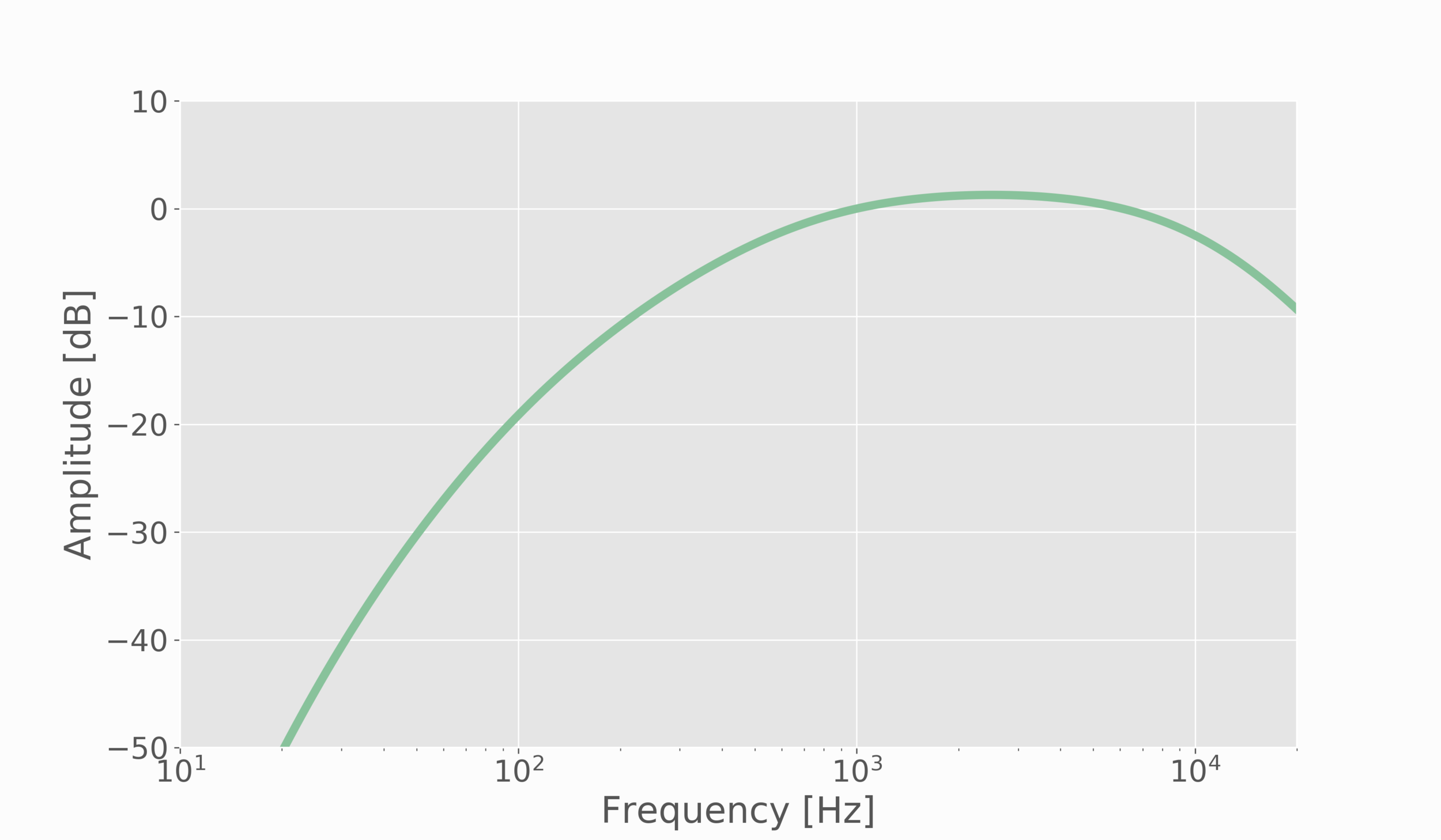
Figure 4: A-weighting function in decibels, used to weight sound measurements to appeal to the human auditory system.
When using the weighting function, we will add the weighted values in decibels at specific frequencies to the measured data in decibels, then convert the new values back to Pascals, sum up the values in each frequency band, then convert that singular number back to decibels for an A-weighted sound pressure level, which is represented as dBA.
import matplotlib.pyplot as plt
import numpy as np
import time,wave

plt.style.use('ggplot')
plt.rcParams['font.size']=18

samp_rate = 44100 # 44.1kHz sampling rate
chunk = 44100 # 2^12 samples for buffer

# compute weighting function
f_vec = samp_rate*np.arange(chunk/2)/chunk # frequency vector based on window size and sample rate

f_vec = f_vec[1:]
R_a = ((12194.0**2)*np.power(f_vec,4))/(((np.power(f_vec,2)+20.6**2)*np.sqrt((np.power(f_vec,2)+107.7**2)*(np.power(f_vec,2)+737.9**2))*(np.power(f_vec,2)+12194.0**2)))

# plot
fig = plt.figure(figsize=(12,7))
ax = fig.add_subplot(111)

plt.plot(f_vec,20*np.log10(R_a)+2.0,linewidth=5,c='#88C29B')
plt.xlabel('Frequency [Hz]')
plt.ylabel('Amplitude [dB]')
plt.grid(True)

ax.set_xlim([10,20000])
ax.set_ylim([-50,10])
ax.set_xscale('log')

plt.savefig('a_weighting_dB.png',dpi=300,facecolor='#FCFCFC')
plt.show()
Sound Pressure Levels
One widely used term in acoustics, specifically with regard to pressure measurement, is the decibel. Acoustically speaking, the decibel is a logarithmic conversion at a reference pressure level, usually 20 micro-Pascals. This can be written as follows:
The P1 above is the converted pressure level from the microphone voltage. Once we convert the pressure to decibels using the equation above, we can compute the A-weighted distribution and finally calculate the average A-weighted sound pressure level - something that is used to define noise pollution and harmful acoustic environments.
I recorded one second of white noise using a smartphone (iPhone X) to measure the accuracy of the microphone and my Python sound pressure level (SPL) calculations. The study I mentioned above (link) measured the iPhone 6 at about 105 dBA. I put the iPhone X on the highest volume with white noise playing and I calculated 102 dBA (reference pressure 20 uPa, measured within inches of the microphone). The recorded white noise is below:
import pyaudio
import matplotlib.pyplot as plt
import numpy as np
import time

plt.style.use('ggplot')
plt.rcParams['font.size']=18

form_1 = pyaudio.paInt16 # 16-bit resolution
chans = 1 # 1 channel
samp_rate = 44100 # 44.1kHz sampling rate
chunk = 44100 # 2^12 samples for buffer
dev_index = 2 # device index found by p.get_device_info_by_index(ii)

audio = pyaudio.PyAudio() # create pyaudio instantiation

# create pyaudio stream
stream = audio.open(format = form_1,rate = samp_rate,channels = chans, \
                    input_device_index = dev_index,input = True, \
                    frames_per_buffer=chunk)

# record data chunk
stream.start_stream()
data = np.fromstring(stream.read(chunk),dtype=np.int16)
stream_data = data
stream.stop_stream()

# mic sensitivity correction and bit conversion
mic_sens_dBV = 47.0 # mic sensitivity in dBV + any gain
mic_sens_corr = np.power(10.0,mic_sens_dBV/20.0) # calculate mic sensitivity conversion factor

# (USB=5V, so 15 bits are used (the 16th for negatives)) and the manufacturer microphone sensitivity corrections
data = ((data/np.power(2.0,15))*5.25)/(mic_sens_corr)

# compute FFT parameters
f_vec = samp_rate*np.arange(chunk/2)/chunk # frequency vector based on window size and sample rate
mic_low_freq = 100 # low frequency response of the mic (mine in this case is 100 Hz)
low_freq_loc = np.argmin(np.abs(f_vec-mic_low_freq))
fft_data = (np.abs(np.fft.fft(data))[0:int(np.floor(chunk/2))])/chunk
fft_data[1:] = 2*fft_data[1:]

max_loc = np.argmax(fft_data[low_freq_loc:])+low_freq_loc

# plot
fig = plt.figure(figsize=(12,6))
ax = fig.add_subplot(111)
plt.plot(f_vec,fft_data)
ax.set_ylim([0,2*np.max(fft_data)])
plt.xlabel('Frequency [Hz]')
plt.ylabel('Amplitude [Pa]')
plt.grid(True)
plt.annotate(r'$\Delta f_{max}$: %2.1f Hz' % (samp_rate/(2*chunk)),xy=(0.7,0.92),\
             xycoords='figure fraction')
annot = ax.annotate('Freq: %2.1f'%(f_vec[max_loc]),xy=(f_vec[max_loc],fft_data[max_loc]),\
                    xycoords='data',xytext=(0,30),textcoords='offset points',\
                    arrowprops=dict(arrowstyle="->"),ha='center',va='bottom')

ax.set_xscale('log')
plt.tight_layout()
plt.savefig('fft_real_signal.png',dpi=300,facecolor='#FCFCFC')
plt.show()

# A-weighting function and application
f_vec = f_vec[1:]
R_a = ((12194.0**2)*np.power(f_vec,4))/(((np.power(f_vec,2)+20.6**2)*np.sqrt((np.power(f_vec,2)+107.7**2)*(np.power(f_vec,2)+737.9**2))*(np.power(f_vec,2)+12194.0**2)))
a_weight_data_f = (20*np.log10(R_a)+2.0)+(20*np.log10(fft_data[1:]/0.00002))
a_weight_sum = np.sum(np.power(10,a_weight_data_f/20)*0.00002)
print(20*np.log10(a_weight_sum/0.00002))
iPhone X Max Sound Pressure Level = 102 dBA
Conclusion
In this entry in the acoustic signal processing series, I discussed in-depth the importance of sampling windows and interpreting real data using a microphone and its specifications. I was using a cheap USB microphone to analyze known signals (1 kHz sine wave, and white noise) to understand how the Fast Fourier Transform processes acoustic signals. Finally, I introduced weighting functions and the decibel along with their significance to the human auditory system. At this point in the acoustics series, the user should be capable of recording and analyzing acoustic signals with some physical significance, primarily limited by the resolution of the microphone and recording system (Raspberry Pi and Python). That being said, we were able to closely replicate the performance of the iPhone under similar test conditions of a previous study analyzing the peak volume of the device. In the next entry of the acoustic signal processing series, I will discuss updating periodograms and frequency spectrum plots for changing acoustic systems.
See More in Audio and Python: