Audio Processing in Python Part I: Sampling, Nyquist, and the Fast Fourier Transform
Since the publication of Joseph Fourier’s groundbreaking paper in 1822 [see page 525 in text], the use of the Fourier Series has been widespread in applications of engineering ranging from heat transfer to vibration analysis. And more recently, after the evolution of computation and algorithms, the use of the Fast Fourier Transform (FFT) has also become ubiquitous in applications ranging from acoustic analysis to turbulence research and modeling. The notion that sine and cosine waves can be combined to create complex real-world signals is the basis for most of the digital signals that we observe in technology today. In this tutorial, I will describe the basic process for emulating a sampled signal and then processing that signal using the FFT algorithm in Python. This will allow the user to get started with analysis of acoustic-like signals and understand the fundamentals of the Fast Fourier Transform.

Jean-Baptiste Joseph Fourier - Creator of the Fourier Series
Fourier Series
The Fast Fourier Transform, proposed by Cooley and Tukey in 1965, is an efficient computational algorithm of the Discrete Fourier Transform (DFT). The DFT decomposes a signal into a series of the following form:
where xm is a point in the signal being analyzed and the Xk is a specific 'mode' or frequency component. Notice that the frequency component can only go up to the length of the signal (M-1), and we will discuss a little later the limitations from there as well (Nyquist).
From above, the complex exponential can be rewritten as sine and cosine functions using the Euler formula:
Such that our series contains sinusoidal waves:
We can now see how a signal can be transformed into a series of sinusoidal waves.
Sine Wave Sampling
The easiest way to test an FFT in Python is to either measure a sinusoidal wave at a known frequency using a microphone, or create a sinusoidal function in Python. Since this section focuses on understanding the FFT, I will demonstrate how to emulate a sampled sine wave using Python. Below is the creation of a sine wave in Python using sampling criteria that emulates a real signal:
# sampling a sine wave programmatically
import numpy as np
import matplotlib.pyplot as plt
plt.style.use('ggplot')

# sampling information
Fs = 44100 # sample rate
T = 1/Fs # sampling period
t = 0.1 # seconds of sampling
N = Fs*t # total points in signal

# signal information
freq = 100 # in hertz, the desired natural frequency
omega = 2*np.pi*freq # angular frequency for sine waves

t_vec = np.arange(N)*T # time vector for plotting
y = np.sin(omega*t_vec)

plt.plot(t_vec,y)
plt.show()
The code above ‘samples’ a sine wave at 44.1 kHz for 0.1 seconds (100 ms). I used a 100 Hz sine wave, so we expect:
This means that we will get 10 cycles from the 100 Hz sine wave in 0.1 seconds. This also means that we will have 4410 samples for the 10 cycles, or 441 samples per cycle - which is quite a bit for replication of the signal. The plot produced by the code is shown below:
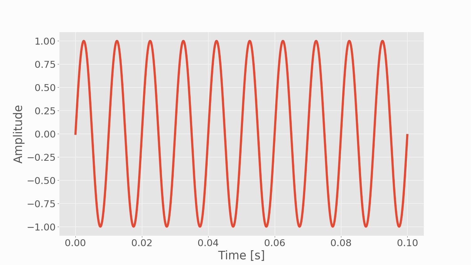
Figure 1: 100 Hz sine wave sampled at 44.1 kHz for 0.1 seconds.
The Nyquist Frequency
In digital signal processing:
"In order to recover all Fourier components of a periodic waveform, it is necessary to use a sampling rate fs at least twice the highest waveform frequency"
The above statement requires the user to sample a signal at twice the highest natural frequency of the expected system, or mathematically:
Therefore, in the FFT function, the limitation of the frequency component is set by the sample rate, which is typically a little higher than twice the highest natural frequency expected in the system. In the case of acoustics, the sample rates are set at approximately twice the highest frequency that humans are capable of discerning (20 kHz), so the sample rate for audio is at minimum 40 kHz. We often see 44.1 kHz or 48 kHz, which means audio is often sampled correctly above the Nyquist frequency set by the range of the human ear. Therefore, in practice, it is essential to adhere to the following inequality:
As a visualization tool, below I have plotted several sampled signals that are sampled around the Nyquist frequency for a 100 Hz sine wave. According to the statement above, if a 100 Hz sine wave is the largest frequency in the system, we should be sampling above 200 Hz.
Figure 2: Plot showing the affects of aliasing around the Nyquist frequency. As the sample rate dips below twice the natural frequency, we start to see the inability to replicate the true signal. In this case, a 100 Hz sine wave was inputted, and at 10 times the Nyquist frequency the signal is clearly replicated. At 1.2 times the Nyquist frequency the signal can still be reconstructed, however, once we dip below twice the natural frequency, or below the Nyquist frequency, we can no longer replicate the original 100 Hz signal.
The phenomena above, when sampling under the Nyquist frequency is called aliasing. Aliasing can obscure measurements and introduce false peaks in data that can result in inaccurate results. This is why we must sample above the highest natural frequency of the system. Of course, some situations do not warrant pre-determined knowledge of the system, but in those cases methods such as time domain filtering can account for such unexpected behavior. Fortunately, in the field of acoustics, we often don’t need to worry about high frequencies above the typical human hearing range (an exception, of course, is in the ultrasonic range).
From here, we can investigate the Fast Fourier Transform (FFT) in Python by using our test signal above and the FFT function in Python
Fast Fourier Transform
This section is informative for two reasons:
we can verify that the sine wave above is sampled correctly
we can gain confidence in our FFT usage by inputting and analyzing a known signal
Now, if we use the example above we can compute the FFT of the signal and investigate the frequency content with an expectation of the behavior outlined above. The Python FFT function in Python is used as follows:
np.fft.fft(signal)
However, it is important to note that the FFT does not produce an immediate physical significance. So we need to divide by the length of the signal, and only take half of the data (single-sided spectrum - not discussed here). From there we need to take the absolute value of the signal to ensure that no imaginary (complex, non-physical) values are present.
The full FFT algorithm and frequency spectrum plot is shown below:
# fourier transform and frequency domain
#
Y_k = np.fft.fft(y)[0:int(N/2)]/N # FFT function from numpy
Y_k[1:] = 2*Y_k[1:] # need to take the single-sided spectrum only
Pxx = np.abs(Y_k) # be sure to get rid of imaginary part

f = Fs*np.arange((N/2))/N; # frequency vector

# plotting
fig,ax = plt.subplots()
plt.plot(f,Pxx,linewidth=5)
ax.set_xscale('log')
ax.set_yscale('log')
plt.ylabel('Amplitude')
plt.xlabel('Frequency [Hz]')
plt.show()
The code takes the FFT of an input signal y (in our case, the sine wave above), which has a length N. It also computes the frequency vector using the number of points and the sampling frequency.
The frequency vector and amplitude spectrum produce the following plot below:
Figure 3: Computed FFT showing the amplitude spectrum of a 100 Hz sine wave.
If we were to analyze the frequency and amplitude at the peak of the spectrum plot above (sometimes called a periodogram), we could conclude that the peak is 3 and the frequency is 100 Hz. This returns the amplitude and frequency of our inputted sine wave. Also note the introduction of noise into the signal. The noise is considered an artifact of the computation and is near to zero, so we can neglect it (its amplitude is 10 to the power -17, so this is a fair assumption). The prediction in this case isn’t particularly impressive, as we could plainly see that the time series above produced a single sine wave at 100 Hz. Below I introduce a more complex signal with three sine waves and some Gaussian noise:
Figure 4: Computed FFT for three separate sine waves at three different amplitudes and frequencies with some added noise. The FFT has trouble resolving one frequency because the sampling period is likely too short. That, in conjunction with the added noise makes resolving the peak more difficult. The other two signals, however, are high enough above the noise that their peaks are more easily resolved.
It may or may not be obvious to the viewer, but the time series above cannot easily be decomposed into any specific frequency. However, after taking the FFT of the signal, we can easily see there are three resolvable peaks. The noise may have obscured the lowest amplitude signal (around the 150 Hz range), and this is normal for noisy signals. We could conclude, without knowing the original sine wave frequencies or amplitudes, that we had three signals:
100 Hz signal at an amplitude of 3
150 Hz signal at an amplitude of 1.5
280 Hz signal at an amplitude of 4.5
The true inputs were: 100 Hz at an amplitude of 3, 155 Hz at an amplitude of 2, 283 Hz at an amplitude of 5.2, and Gaussian noise at an amplitude of 1. Notice the error associated with the FFT upon introduction of noise. This is important to keep in mind when analyzing signals using FFTs. One way to reduce the error is to record the signal for longer or try to get the recording device closer to the source (or increase the amplitude of the signal). Occasionally, neither of these methods are possible, which is when other techniques need to be employed such as windowing or time/frequency filtering. I will not cover those more complex signal processing methods here, but if the user is interested in learning about windowing or time/frequency filters, please see the following references: here, here, and here.

Figure 5: Visual breakdown showing a complex signal being decomposed into its parts (3 sine wave, and some Gaussian noise). The last plot is the FFT of the singular complex signal, indicating the three individual sine waves at their respective frequency locations and amplitudes.
Conclusion and Continuation
In this tutorial, I discussed sampling and the Fast Fourier Transform and their relation to signal processing with the intention of creating a series on audio signal processing and the Raspberry Pi. Digital signal processing is one of the most important fields in technology today, and the FFT maintains a firm hold on signal analysis in the digital domain. Above, I demonstrated how to create a sampled signal and then process it using Python’s FFT function to find the peaks and amplitudes. The FFT is such a powerful tool because it allows the user to take an unknown signal a domain and analyze it in the frequency domain to gain information about the system. In the next entry of the Audio Processing in Python series, I will discuss analysis of audio data using the Python FFT function. I will also introduce windowing, sound pressure levels, and frequency weighting. The next entry will focus on physical significance of microphone data to enable the user to analyze pressure data as well as frequency information for use in relation to the human auditory system.
See More in Acoustics and Engineering: