Introduction
Installing Anaconda 3 and Cartopy
Street Map Cartopy Visualizations
Scatter Points Atop a Map
Conclusion

Cartopy is a cartographic Python library, hence its naming convention, that was developed for applications in geographic data manipulation and visualization. It is the successor to the the Basemap Toolkit, which was the previous Python library used for geographic visualizations (several Basemap tutorials can be found on our site: Geographic Mapping from a CSV File, Satellite Imagery Analysis, GOES-16 Latitude/Longitude Projection Algorithm). Cartopy can be used to plot satellite data atop realistic maps, visualize city and country boundaries, track and predict movement based on geographic targeting, and a range of other applications relating to geographic-encoded data systems. In this tutorial, Anaconda 3 will be used to install Cartopy and related geographic libraries. As an introduction to the library and geographic visualizations, some simple tests will be conducted to ensure that the Cartopy library was successfully installed and is working properly. In subsequent tutorials: shapefiles will be used as boundaries, realistic city streets will be mapped, and satellite data will be analyzed.

Installing Anaconda 3 and Cartopy

Anaconda 3 is chosen as the Python platform because of its robust handling of Python libraries and packages. It is free, open-source, and dynamically manages packages as new ones are installed. This is particularly important for complex libraries such as Cartopy, which requires a wide range of prerequisites. Another recommendation is that either Mac or Linux are used with Cartopy. The reason being - some of the Python libraries struggle with Windows platforms due to issues with environment variables, programmatic navigation, and administrative permissions. Thus, it is strongly recommended that either Linux or Mac operating systems are used.

Installing Anaconda 3

The following install process is for the terminal-based install of Anaconda 3 from a Linux operating system (Ubuntu 19.x is used here):

1. Download Anaconda 3 from (Python 3.x version): https://www.anaconda.com/distribution/#download-section

2. Once the download finishes, navigate to the folder where it downloaded and type:

3. Next, the installer will ask the user to agree to the terms, click enter and type yes when prompted. For the full download procedure, go to the Anaconda page and follow their instructions: https://docs.anaconda.com/anaconda/install/linux/. The defaults will be used here going forward (agreeing to all terms and default initializations).

4. Once the install reaches the “Thank you for installing Anaconda3” - close the terminal

5. Upon reopening the terminal, type the following:

6. Next, ensure that conda has been installed by looking at the current environments in Anaconda 3 by typing:

At this point, Anaconda 3 should be installed on the local system and the above should have printed out the following:

This means that the base Anaconda 3 environment has been installed.

Installing Cartopy and Dependencies

What we need to do now is create an entirely new environment and tailor it to the Cartopy library and dependencies. The Anaconda team has a cheat sheet which is very useful when creating, updating, and navigating through environments in Anaconda, which can be found here. There, users can find quick terminal commands to create and alter environments. In the case of Cartopy, the first command will involve creating a Cartopy environment called ‘cartopy_env’ which will contain all of the necessary libraries for geographic mapping:

The first command installs the environment ‘cartopy_env’ and uses ‘conda-forge’ as the install channel. Using ‘conda-forge’ allows the user to maintain libraries in an Anaconda environment in a dynamic way, without installing conflicting or incompatible libraries or versions.

Once the new environment is created, it must be activated. Type and run the following command into the terminal:

The user should now see an updated terminal line that has the new environment active, which should look similar to the following:

To verify the current environment, type the following:

This should output the current active environment with an asterisk *:

If the asterisk is next to the new environment, ‘cartopy_env,’ then the install process is complete and the correct environment has been installed. Next, the Jupyter Lab can be installed, to make programming in Python more versatile. Jupyter Lab is a GUI that works via a web interface and is connected to the Jupyter Notebook family, making it a great tool for real-time visualizations and coding. The Jupyter framework can be downloaded with the following command, under the assumption that ‘cartopy_env’ is active:

The above command will use ‘conda-forge’ again to install the Jupyter Lab and Jupyter Notebook dependencies. This general command should be used when installing any new libraries needed when using the environment:

conda install -c conda-forge ______

This formality will keep all libraries on the same channel and prevent any conflicts or incompatibilities. Once the Jupyter Lab download is complete, start it by typing the following under the active ‘cartopy_env’:

Jupyter Lab should now open in the user’s local web browser and appear similar to the following:

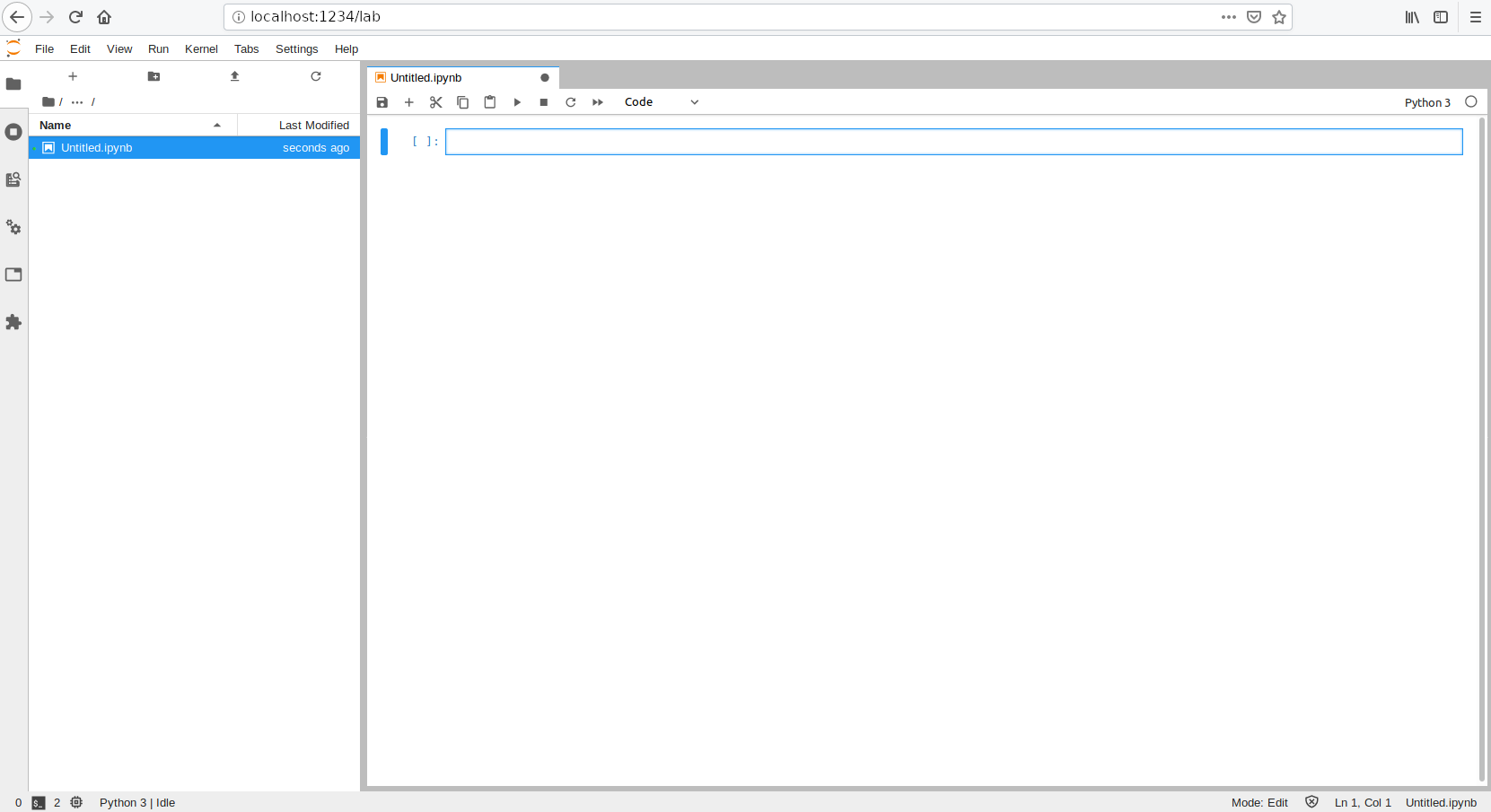
At this point, Anaconda 3 and Cartopy are ready for testing. The install of Cartopy can be further verified by typing in ‘import cartopy.crs as ccrs’ - and if there are no errors following the run of the script, then the library and environment are verified! A short introduction to Cartopy is given in the next section.

Street Map Cartopy Visualizations

Jupyter Lab will be used in this section to output visualizations produced by Cartopy. The simplest starting point when dealing with a new software is to attempt examples that relate to known conditions. The Maker Portal team is located in New York City (NYC), thus, the example below uses the location of the One World Trade Center (40.713, -74.0135) to map the surrounding area in New York City using an open street map (OSM) and Cartopy:

# Mapping New York City Open Street Map (OSM) with Cartopy
# This code uses a spoofing algorithm to avoid bounceback from OSM servers
#
import matplotlib.pyplot as plt 
import numpy as np
import cartopy.crs as ccrs
import cartopy.io.img_tiles as cimgt
import io
from urllib.request import urlopen, Request
from PIL import Image

def image_spoof(self, tile): # this function pretends not to be a Python script
    url = self._image_url(tile) # get the url of the street map API
    req = Request(url) # start request
    req.add_header('User-agent','Anaconda 3') # add user agent to request
    fh = urlopen(req) 
    im_data = io.BytesIO(fh.read()) # get image
    fh.close() # close url
    img = Image.open(im_data) # open image with PIL
    img = img.convert(self.desired_tile_form) # set image format
    return img, self.tileextent(tile), 'lower' # reformat for cartopy

cimgt.OSM.get_image = image_spoof # reformat web request for street map spoofing
osm_img = cimgt.OSM() # spoofed, downloaded street map

fig = plt.figure(figsize=(12,9)) # open matplotlib figure
ax1 = plt.axes(projection=osm_img.crs) # project using coordinate reference system (CRS) of street map
center_pt = [40.713, -74.0135] # lat/lon of One World Trade Center in NYC
zoom = 0.00075 # for zooming out of center point
extent = [center_pt[1]-(zoom*2.0),center_pt[1]+(zoom*2.0),center_pt[0]-zoom,center_pt[0]+zoom] # adjust to zoom
ax1.set_extent(extent) # set extents

scale = np.ceil(-np.sqrt(2)*np.log(np.divide(zoom,350.0))) # empirical solve for scale based on zoom
scale = (scale<20) and scale or 19 # scale cannot be larger than 19
ax1.add_image(osm_img, int(scale)) # add OSM with zoom specification
# NOTE: zoom specifications should be selected based on extent:
# -- 2     = coarse image, select for worldwide or continental scales
# -- 4-6   = medium coarseness, select for countries and larger states
# -- 6-10  = medium fineness, select for smaller states, regions, and cities
# -- 10-12 = fine image, select for city boundaries and zip codes
# -- 14+   = extremely fine image, select for roads, blocks, buildings
plt.show() # show the plot

The resulting output in the Jupyter Lab Notebook should be identical to the following:

The map outputted above is at the highest resolution possible with the Open Street Map (OSM). If we were to zoom out a little from the point, we would see a different scale set. The scale can be customized, but as the scale increases, so does the time it takes to plot the map. This is why the automatic scale function is added.

Let’s try another type of map called 'QuadtreeTiles' - which is a photo-realistic depiction of the surface. For example, if we substitute 'QuadtreeTiles' in place of 'OSM' in the code above, we get the following snapshot of the One World Trade Center:

one_world_trade_nyc_map_zoom_scale_19_quadtreetiles.jpg

The successful city visualizations above indicate that Anaconda 3 is working, Cartopy has been successfully installed, and that our tests are accurate and reproducible. A quick Google search of One World Trade Center indicates that the snapshots above are accurate and somewhat mirror the visuals present on Google Maps (excluding any updates that don’t align over the years). In the next section, scatter points of weather stations will be plotted over a map of the U.S. to further explore the capabilities of Cartopy.

Scatter Points Atop A Map

A database of weather stations associated with the Automated Surface Observing System (ASOS) can be found at the following link:

ftp://ftp.ncdc.noaa.gov/pub/data/ASOS_Station_Photos/asos-stations.txt

The ASOS network is a distribution of weather stations that update temperature, humidity, wind direction, precipitation, and other weather information every minute. The ASOS network is primarily used for aircraft and airports to report on weather and safety during takeoff and landing. Moreover, ASOS stations have been used in research related to satellite algorithms, numerical weather prediction, and web-based weather applications. The ASOS .txt file contains 915 stations scattered across the United States and its territories. Starting from row 5 onward, the stations are parsed. There are 14 columns per station, where the latitude and longitude coordinates can be pulled from the 10th and 11th columns. Once the 'asos-stations.txt' file is downloaded, the data can be parsed into Python and used as a tool for finding details about local weather. This will be explored with Cartopy and other Python libraries.

The code below parses the ASOS .txt file and maps the stations across the contiguous United States (sometimes called CONUS):

# Mapping ASOS Weather Stations Across the Contiguous United States
# This code uses a spoofing algorithm to avoid bounceback from OSM servers
# -- This code also parses lat/lon information from the ASOS station .txt
# -- file located here: ftp://ftp.ncdc.noaa.gov/pub/data/ASOS_Station_Photos/asos-stations.txt
#
import csv
import numpy as np
import cartopy.crs as ccrs
import matplotlib.pyplot as plt
import cartopy.io.img_tiles as cimgt
from cartopy.mpl.ticker import LongitudeFormatter, LatitudeFormatter
import io
from urllib.request import urlopen, Request
from PIL import Image

def image_spoof(self, tile): # this function pretends not to be a Python script
    url = self._image_url(tile) # get the url of the street map API
    req = Request(url) # start request
    req.add_header('User-agent','Anaconda 3') # add user agent to request
    fh = urlopen(req) 
    im_data = io.BytesIO(fh.read()) # get image
    fh.close() # close url
    img = Image.open(im_data) # open image with PIL
    img = img.convert(self.desired_tile_form) # set image format
    return img, self.tileextent(tile), 'lower' # reformat for cartopy

################################
# parsing the ASOS coordinates
################################
#
asos_data = []
with open('asos-stations.txt','r') as dat_file:
    reader = csv.reader(dat_file)
    for row in reader:
        asos_data.append(row)

row_delin = asos_data[3][0].split(' ')[:-1]
col_sizes = [len(ii) for ii in row_delin]

col_header = []; iter_ii = 0
for ii,jj in enumerate(col_sizes):
    col_header.append(asos_data[2][0][iter_ii:iter_ii+col_sizes[ii]].replace(' ',''))
    iter_ii+=col_sizes[ii]+1
    
call,names,lats,lons,elevs = [],[],[],[],[]
for row in asos_data[4:]:
    data = []; iter_cc = 0
    for cc in range(0,len(col_header)):
        data.append(row[0][iter_cc:iter_cc+col_sizes[cc]].replace('  ',''))
        iter_cc+=col_sizes[cc]+1
    call.append(data[3])
    names.append(data[4])
    lats.append(float(data[9]))
    lons.append(float(data[10]))
    elevs.append(float(data[11]))

#######################################
# Formatting the Cartopy plot
#######################################
#
cimgt.Stamen.get_image = image_spoof # reformat web request for street map spoofing
osm_img = cimgt.Stamen('terrain-background') # spoofed, downloaded street map

fig = plt.figure(figsize=(12,9)) # open matplotlib figure
ax1 = plt.axes(projection=osm_img.crs) # project using coordinate reference system (CRS) of street map
ax1.set_title('ASOS Station Map',fontsize=16)
extent = [-124.7844079,-66.9513812, 24.7433195, 49.3457868] # Contiguous US bounds
# extent = [-74.257159,-73.699215,40.495992,40.915568] # NYC bounds
ax1.set_extent(extent) # set extents
ax1.set_xticks(np.linspace(extent[0],extent[1],7),crs=ccrs.PlateCarree()) # set longitude indicators
ax1.set_yticks(np.linspace(extent[2],extent[3],7)[1:],crs=ccrs.PlateCarree()) # set latitude indicators
lon_formatter = LongitudeFormatter(number_format='0.1f',degree_symbol='',dateline_direction_label=True) # format lons
lat_formatter = LatitudeFormatter(number_format='0.1f',degree_symbol='') # format lats
ax1.xaxis.set_major_formatter(lon_formatter) # set lons
ax1.yaxis.set_major_formatter(lat_formatter) # set lats
ax1.xaxis.set_tick_params(labelsize=14)
ax1.yaxis.set_tick_params(labelsize=14)

scale = np.ceil(-np.sqrt(2)*np.log(np.divide((extent[1]-extent[0])/2.0,350.0))) # empirical solve for scale based on zoom
scale = (scale<20) and scale or 19 # scale cannot be larger than 19
ax1.add_image(osm_img, int(scale)) # add OSM with zoom specification

#######################################
# Plot the ASOS stations as points
#######################################
#
ax1.plot(lons, lats, markersize=5,marker='o',linestyle='',color='#3b3b3b',transform=ccrs.PlateCarree())

plt.show()

The map outputted by the code is given below:

The scale may appear blurry depending on the size of the screen that is viewing the map. If a higher resolution map is desired, a larger scale factor can be used. Scale factor 4 is used here to keep the load times of this webpage minimal. For the application here, the image above suffices. If the scatter map was being used for publication purposes, it should be scaled up to 6 or even 7 (which results in longer load times and much larger image sizes).

To see stations in a particular area, for example New York City again, the extents can be changed (uncomment the NYC extent above in the code) and the ASOS stations can be observed for a given boundary. And instead of using the 'terrain-background' mapping in the ‘Stamen()’ function, change it to simply: 'terrain.' For the NYC case, this is results in the following:

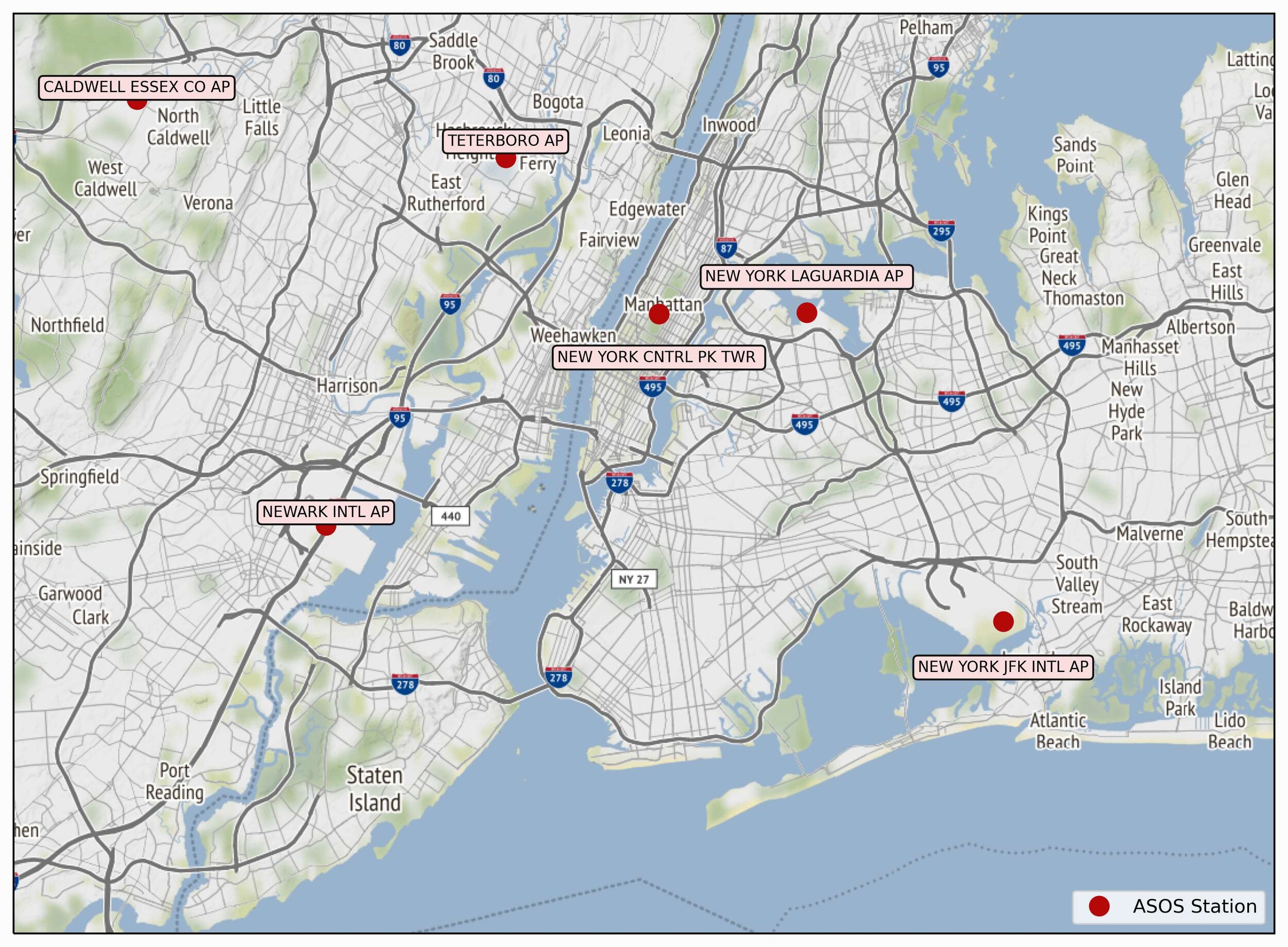
Since the majority of the ASOS stations are located at airports, it’s easy to verify the locations of the stations in New York City. The three large airports: LaGuardia, JFK, Newark - all have red dots above them, as expected. A fourth dot is located at another well-established location: Central Park. The fifth and last ASOS station is located at the Teterboro Airport.

If location is particularly important, text annotations can be added to the map to identify each station. This is done in the plot below:

The code to replicate this plot with text annotations is given below:

# Mapping ASOS Weather Stations Across New York City and Annotating Them
# This code uses a spoofing algorithm to avoid bounceback from OSM servers
# -- This code also parses lat/lon information from the ASOS station .txt
# -- file located here: ftp://ftp.ncdc.noaa.gov/pub/data/ASOS_Station_Photos/asos-stations.txt
#
import csv
import numpy as np
import cartopy.crs as ccrs
import matplotlib.pyplot as plt
import cartopy.io.img_tiles as cimgt
from cartopy.mpl.ticker import LongitudeFormatter, LatitudeFormatter
import io
from urllib.request import urlopen, Request
from PIL import Image

def image_spoof(self, tile): # this function pretends not to be a Python script
    url = self._image_url(tile) # get the url of the street map API
    req = Request(url) # start request
    req.add_header('User-agent','Anaconda 3') # add user agent to request
    fh = urlopen(req) 
    im_data = io.BytesIO(fh.read()) # get image
    fh.close() # close url
    img = Image.open(im_data) # open image with PIL
    img = img.convert(self.desired_tile_form) # set image format
    return img, self.tileextent(tile), 'lower' # reformat for cartopy

################################
# parsing the ASOS coordinates
################################
#
asos_data = []
with open('asos-stations.txt','r') as dat_file:
    reader = csv.reader(dat_file)
    for row in reader:
        asos_data.append(row)

row_delin = asos_data[3][0].split(' ')[:-1]
col_sizes = [len(ii) for ii in row_delin]

col_header = []; iter_ii = 0
for ii,jj in enumerate(col_sizes):
    col_header.append(asos_data[2][0][iter_ii:iter_ii+col_sizes[ii]].replace(' ',''))
    iter_ii+=col_sizes[ii]+1
    
call,names,lats,lons,elevs = [],[],[],[],[]
for row in asos_data[4:]:
    data = []; iter_cc = 0
    for cc in range(0,len(col_header)):
        data.append(row[0][iter_cc:iter_cc+col_sizes[cc]].replace('  ',''))
        iter_cc+=col_sizes[cc]+1
    call.append(data[3])
    names.append(data[4])
    lats.append(float(data[9]))
    lons.append(float(data[10]))
    elevs.append(float(data[11]))

#######################################
# Formatting the Cartopy plot
#######################################
#
cimgt.Stamen.get_image = image_spoof # reformat web request for street map spoofing
osm_img = cimgt.Stamen('terrain') # spoofed, downloaded street map

fig = plt.figure(figsize=(12,9)) # open matplotlib figure
ax1 = plt.axes(projection=osm_img.crs) # project using coordinate reference system (CRS) of street map
ax1.set_title('ASOS Station Map',fontsize=16)
# extent = [-124.7844079,-66.9513812, 24.7433195, 49.3457868] # Contiguous US bounds
extent = [-74.257159,-73.699215,40.495992,40.915568] # NYC bounds
ax1.set_extent(extent) # set extents
ax1.set_xticks(np.linspace(extent[0],extent[1],7),crs=ccrs.PlateCarree()) # set longitude indicators
ax1.set_yticks(np.linspace(extent[2],extent[3],7)[1:],crs=ccrs.PlateCarree()) # set latitude indicators
lon_formatter = LongitudeFormatter(number_format='0.1f',degree_symbol='',dateline_direction_label=True) # format lons
lat_formatter = LatitudeFormatter(number_format='0.1f',degree_symbol='') # format lats
ax1.xaxis.set_major_formatter(lon_formatter) # set lons
ax1.yaxis.set_major_formatter(lat_formatter) # set lats
ax1.xaxis.set_tick_params(labelsize=14)
ax1.yaxis.set_tick_params(labelsize=14)

scale = np.ceil(-np.sqrt(2)*np.log(np.divide((extent[1]-extent[0])/2.0,350.0))) # empirical solve for scale based on zoom
scale = (scale<20) and scale or 19 # scale cannot be larger than 19
ax1.add_image(osm_img, int(scale)) # add OSM with zoom specification

#######################################
# Plot the ASOS stations as points
#######################################
#
ax1.plot(lons, lats, markersize=10,marker='o',linestyle='',color='#b30909',transform=ccrs.PlateCarree(),label='ASOS Station')
transform = ccrs.PlateCarree()._as_mpl_transform(ax1) # set transform for annotations
# text annotations
for lat_s,lon_s,name_s in zip(lats,lons,names): # loop through lats/lons/names
    if lon_s>extent[0] and lon_s<extent[1] and lat_s>extent[2] and lat_s<extent[3]:
        print(name_s)
        # annotations, with some random placement to avoid overlap
        ax1.text(lon_s, lat_s+(np.random.randn(1)*0.01),name_s, {'color': 'k', 'fontsize': 8},
                 horizontalalignment='center', verticalalignment='bottom',
                 clip_on=False,transform=transform,bbox=dict(boxstyle="round",
                   ec='#121212', fc='#fadede'))

ax1.legend() # add a legend 
plt.show() # show plot

Conclusion

Cartopy is a powerful cartographic library that exists as part of Python’s many visualization toolboxes. In this tutorial, the installation procedures were given for Anaconda 3 and Cartopy, tailed to the specific application of geographic mapping on Linux-based systems. In the first application section above, street maps were plotted for given geographic coordinate. The One World Trade center was mapped on two different street maps: one drawn and one imagery-based. In the second application, the Automated Surface Observing System (ASOS) coordinate points were mapped across the contiguous United States to apply real data to Cartopy capabilities. And lastly, the ASOS coordinates were further explored through text annotations in the greater New York City area. Five ASOS coordinates were verified in NYC by looking at the names associated with each coordinate and relating each to the respective nearby airport or weather station. In the upcoming tutorials, Cartopy will continue to be explored, particularly for real-world applications involving shapefiles of cities and satellite data.

Citation for This Page:

See More in GIS and Python:

Featured