How to Create a Rotating Globe Using Python and the Basemap Toolkit

Back to Top

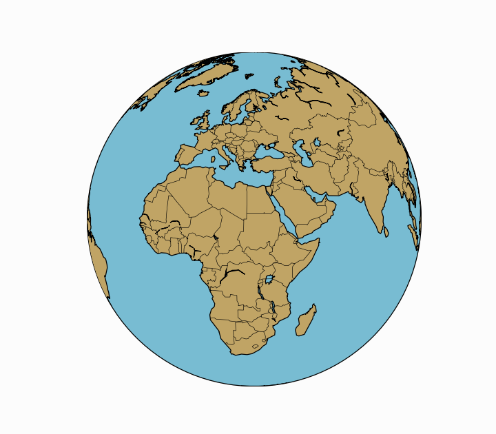
In this tutorial, I will utilize several tools used in previous blog entries. I recommend reviewing how to map with Python's Basemap toolkit, real-time plotting - and if necessary, Python's matplotlib library. I will be using an orthographic projection to visualize earth from an extraterrestrial vantage point, such that, in conjunction with NASA's Blue Marble image, we can resolve realistic contours of earth from space with impressive detail. For visualization purposes, I will also be using a gif-maker function to create a dynamic animation of earth rotating about a specific latitudinal angle. All of this will be accomplished using available libraries installed with Python's Basemap toolkit (except, perhaps the imageio library for making GIFs).

Blog Post Index:

Relevant Past Projects
Viewing Earth Using an Orthographic Projection
Varying the Perspective Angle
Animated GIF of Rotating Earth
Earth Rotating in a Galaxy - High Definition
Conclusion

In previous tutorials I demonstrated multiple data visualization methods using: animated GIFs, live-plotting, geographic mapping, and various tools related to the matplotlib library in Python. For information and further exploration, click any of the links below:

---

Viewing Earth Using an Orthographic Projection

The orthographic projection differs from traditional projections as it does not allow the viewer to see the full surface area of the earth. Consequently, we observe distortion around the edges of the spherical projection, but maintain much of the directional properties of the earth itself. Basemap offers dozens of projection options including cylindrical, conical, and planar. In order to view the globe as a rotating sphere (not spheroid - the best we can do!), we will be using the azimuthal orthographic (planar) projection, which looks something like the image below:

Click for Orthographic Example Code

from mpl_toolkits.basemap import Basemap
import matplotlib.pyplot as plt
import numpy as np

fig = plt.figure(figsize=(9,6))

# set perspective angle
lat_viewing_angle = 50
lon_viewing_angle = -73

# define color maps for water and land
ocean_map = (plt.get_cmap('ocean'))(210)
cmap = plt.get_cmap('gist_earth')

# call the basemap and use orthographic projection at viewing angle
m = Basemap(projection='ortho', 
          lat_0=lat_viewing_angle, lon_0=lon_viewing_angle)    

# coastlines, map boundary, fill continents/water, fill ocean, draw countries
m.drawcoastlines()
m.drawmapboundary(fill_color=ocean_map)
m.fillcontinents(color=cmap(200),lake_color=ocean_map)
m.drawcountries()

# latitude/longitude line vectors
lat_line_range = [-90,90]
lat_lines = 8
lat_line_count = (lat_line_range[1]-lat_line_range[0])/lat_lines

merid_range = [-180,180]
merid_lines = 8
merid_count = (merid_range[1]-merid_range[0])/merid_lines

m.drawparallels(np.arange(lat_line_range[0],lat_line_range[1],lat_line_count))
m.drawmeridians(np.arange(merid_range[0],merid_range[1],merid_count))

# save figure at 150 dpi and show it
plt.savefig('orthographic_map_example_python.png',dpi=150,transparent=True)
plt.show()

Using the code above, we can introduce a loop and rotation scheme that simulates a rotating globe. In the next section, I introduce rotation by varying the perspective angle. 

---

Varying the Perspective Angle

To vary the perspective and begin the illusion of a rotating earth, we only need to change one variable: the longitudinal viewing angle. We can, of course, vary both latitude and longitude, but to create a realistic rotation of earth, we need to fix the latitudinal viewing angle and rotate the longitudinal viewing angle. This can be done by altering the perspective angle in the code above:

# set perspective angle
lat_viewing_angle = 45.4642
lon_viewing_angle = 9.1900

In this case, I chose Milan, Italy as the central viewing coordinate. The respective orthographic map looks like the following:

Click for Perspective Angle and Zoom Example Code

from mpl_toolkits.basemap import Basemap
import matplotlib.pyplot as plt
import numpy as np

fig = plt.figure(figsize=(7,6))

# set perspective angle
lat_viewing_angle = 45.4642
lon_viewing_angle = 9.1900

# define color maps for water and land
ocean_map = (plt.get_cmap('ocean'))(210)
cmap = plt.get_cmap('gist_earth')

# call the basemap and use orthographic projection at viewing angle
m1 = Basemap(projection='ortho',
          lat_0=lat_viewing_angle,lon_0=lon_viewing_angle,resolution=None)

# define map coordinates from full-scale globe
map_coords_xy = [m1.llcrnrx,m1.llcrnry,m1.urcrnrx,m1.urcrnry]
map_coords_geo = [m1.llcrnrlat,m1.llcrnrlon,m1.urcrnrlat,m1.urcrnrlon]

#zoom proportion and re-plot map 
zoom_prop = 7.0 # use 1.0 for full-scale map

m = Basemap(projection='ortho',resolution='l',
          lat_0=lat_viewing_angle,lon_0=lon_viewing_angle,llcrnrx=-map_coords_xy[2]/zoom_prop,
            llcrnry=-map_coords_xy[3]/zoom_prop,urcrnrx=map_coords_xy[2]/zoom_prop,
            urcrnry=map_coords_xy[3]/zoom_prop)

# coastlines, map boundary, fill continents/water, fill ocean, draw countries
m.drawmapboundary(fill_color=ocean_map)
m.fillcontinents(color=cmap(200),lake_color=ocean_map)
m.drawcoastlines()
m.drawcountries()

# latitude/longitude line vectors
lat_line_range = [-90,90]
lat_lines = 8
lat_line_count = (lat_line_range[1]-lat_line_range[0])/lat_lines

merid_range = [-180,180]
merid_lines = 8
merid_count = (merid_range[1]-merid_range[0])/merid_lines

m.drawparallels(np.arange(lat_line_range[0],lat_line_range[1],lat_line_count))
m.drawmeridians(np.arange(merid_range[0],merid_range[1],merid_count))

# scatter to indicate lat/lon point
x,y = m(lon_viewing_angle,lat_viewing_angle)
m.scatter(x,y,marker='o',color='#DDDDDD',s=3000,zorder=10,alpha=0.7,\
          edgecolor='#000000')
m.scatter(x,y,marker='o',color='#000000',s=100,zorder=10,alpha=0.7,\
          edgecolor='#000000')

plt.annotate('Milan, Italy', xy=(x, y),  xycoords='data',
                xytext=(-110, -10), textcoords='offset points',
                color='k',fontsize=12,bbox=dict(facecolor='w', alpha=0.5),
                arrowprops=dict(arrowstyle="fancy", color='k'),
                zorder=20)

# save figure at 150 dpi and show it
plt.savefig('ortho_zoom_example.png',dpi=150,transparent=True)
plt.show()

With the ability to alter the perspective angle, we can now loop through an array of chosen longitudinal view points to simulate a rotating globe.

---

Animated GIF of Rotating Earth

In a previous tutorial, I introduced a function that saves a series of .png files and loops through them to create animated GIFs [review the function here]. In this section, I will be using that function (gifly) to create the illusion of a rotating earth. By varying the longitudinal perspective angle, the simple rotating earth GIF is created using the code outlined below.

The animation takes roughly 2 minutes and 40 seconds to run on a Macbook with 8GB RAM and a 2GHz i7 processor. The function is not necessarily a real-time animation, however, the GIF runs smoothly and occupies roughly 10MB of space. The animation runs on all platforms and is a great addition to presentations and lectures without needing to worry about file formats.

Additionally, it is important to note the import of the GIF function:

from gifly import gif_maker

This function should be in the same folder as the script used to create the animated GIF. I have uploaded the 'gifly' function on this project's GitHub page [download it here].

Click for Rotating Earth GIF Example Code

import datetime,matplotlib,time
from mpl_toolkits.basemap import Basemap
import matplotlib.pyplot as plt
import numpy as np
from gifly import gif_maker

# plt.ion() allows python to update its figures in real-time
plt.ion()
fig = plt.figure(figsize=(9,6))

# set the latitude angle steady, and vary the longitude. You can also reverse this to
# create a rotating globe latitudinally as well
lat_viewing_angle = [20.0,20.0]
lon_viewing_angle = [-180,180]
rotation_steps = 150
lat_vec = np.linspace(lat_viewing_angle[0],lat_viewing_angle[0],rotation_steps)
lon_vec = np.linspace(lon_viewing_angle[0],lon_viewing_angle[1],rotation_steps)

# for making the gif animation
gif_indx = 0

# define color maps for water and land
ocean_map = (plt.get_cmap('ocean'))(210)
cmap = plt.get_cmap('gist_earth')

# loop through the longitude vector above
for pp in range(0,len(lat_vec)):    
    plt.cla()
    m = Basemap(projection='ortho', 
              lat_0=lat_vec[pp], lon_0=lon_vec[pp])
    
    # coastlines, map boundary, fill continents/water, fill ocean, draw countries
    m.drawmapboundary(fill_color=ocean_map)
    m.fillcontinents(color=cmap(200),lake_color=ocean_map)
    m.drawcoastlines()
    m.drawcountries()

    #show the plot, introduce a small delay to allow matplotlib to catch up
    plt.show()
    plt.pause(0.01)
    # iterate to create the GIF animation
    gif_maker('basemap_rotating_globe.gif','./png_dir/',gif_indx,len(lat_vec)-1,dpi=90)
    gif_indx+=1

At this point in the tutorial, the user should be capable of producing the rotating globe shown above. Many of the parameters are tunable: latitude viewing angle, frame rate, land color, ocean color, resolution of latitudinal frame (rotation steps), etc. This gives the user the ability to create a wide array of applications relating to earth animations with Python's Basemap toolkit. From here, I will demonstrate how to insert the rotating globe into a space backdrop, and also include NASA's high resolution Blue Marble image to create a realistic depiction of a rotating earth from an outer space perspective angle.

---

Earth Rotating in a Galaxy - High Definition

We can take the animation a step further by placing a background behind the globe to simulate a space-like environment. To do so, I downloaded a .png image of space [this one] and placed it on a parallel axis behind the Basemap image. Additionally, I used NASA's Blue Marble image which provides realistic contours and colors of earth. These two improvements create the animation shown here.

Click for Rotating Earth GIF Example Code

import datetime,matplotlib,time
from mpl_toolkits.basemap import Basemap
import matplotlib.pyplot as plt
import numpy as np
from gifly import gif_maker

plt.ion()
fig,ax0 = plt.subplots(figsize=(5.3,4))
ax0.set_position([0.0,0.0,1.0,1.0])

lat_viewing_angle = [20,20]
lon_viewing_angle = [-180,180]
rotation_steps = 150
lat_vec = np.linspace(lat_viewing_angle[0],lat_viewing_angle[0],rotation_steps)
lon_vec = np.linspace(lon_viewing_angle[0],lon_viewing_angle[1],rotation_steps)

m1 = Basemap(projection='ortho', 
          lat_0=lat_vec[0], lon_0=lon_vec[0],resolution=None)

# add axis for space background effect
galaxy_image = plt.imread('galaxy_image.png')
ax0.imshow(galaxy_image)
ax0.set_axis_off()
ax1 = fig.add_axes([0.25,0.2,0.5,0.5])

# define map coordinates from full-scale globe
map_coords_xy = [m1.llcrnrx,m1.llcrnry,m1.urcrnrx,m1.urcrnry]
map_coords_geo = [m1.llcrnrlat,m1.llcrnrlon,m1.urcrnrlat,m1.urcrnrlon]

#zoom proportion and re-plot map 
zoom_prop = 2.0 # use 1.0 for full-scale map

gif_indx = 0
for pp in range(0,len(lat_vec)):

    ax1.clear()
    ax1.set_axis_off()
    m = Basemap(projection='ortho',resolution='l',
              lat_0=lat_vec[pp],lon_0=lon_vec[pp],llcrnrx=-map_coords_xy[2]/zoom_prop,
                llcrnry=-map_coords_xy[3]/zoom_prop,urcrnrx=map_coords_xy[2]/zoom_prop,
                urcrnry=map_coords_xy[3]/zoom_prop)

    m.bluemarble(scale=0.5)
    m.drawcoastlines()
    plt.show()
    plt.pause(0.01)
    gif_maker('blue_marble_rotating_globe.gif','./png_dir_bluemarble/',gif_indx,len(lat_vec)-1,dpi=90)
    gif_indx+=1

The full code takes between 8-10 minutes to run with a Blue Marble resolution is 50% (on my particular machine, referenced above). As far as I know, the routine above is the most efficient way to create the .gif of the animated Basemap plot. A preferred method for this type of animation would be rotation of the map, however, I do not believe the ability to do that exists under the Basemap toolkit.

NOTE on Resolution:

The .gif file may be quite large depending on the chosen Blue Marble resolution and the size of the plot area (figure size) as well as the background image resolution. Keep this in mind when setting the figure size, resolution step, frame rate, etc. In on case, I produced a 64MB high resolution .gif that was the resolution of my screen.

---

Conclusion

In this tutorial, I outlined the creation of a rotating globe using Python's Basemap toolkit in conjunction with NASA's Blue Marble image. I introduced orthographic projection  in Python and the idea of perspective viewpoints, which allowed us to view the globe from an extraterrestrial vantage point. By varying the longitudinal viewing angle, we were able to create the illusion of a rotating globe. Many factors affect the performance and visuals of the rotating globe: the revolution step, frame rate, figure size, Blue Marble resolution - all of which are alterable depending on the desired outcome for the .gif image. A few applications using this project: a rotating globe for a presentation on geography; a rotating globe for visualization of an array of multi-continental destinations; an animation for satellite view angles; an animation for solar radiation purposes...the possibilities are numerous! I plan to use this project to map airport destinations in real-time based on flight departure times - so stay tuned for that application.

Resources: 

• https://basemaptutorial.readthedocs.io/en/latest/plotting_data.html

• https://matplotlib.org/basemap/users/ortho.html

• https://jakevdp.github.io/PythonDataScienceHandbook/04.13-geographic-data-with-basemap.html

---

See More in Programming and Python: