Listening to Your Pipes with a MEMS Microphone and Raspberry Pi

Water consumption is almost universally measured using a device placed inline with the user's piping system. This requires invasive plumbing and can be costly and disturbing to the user's daily routine. Additionally, common water meters have moving parts that degrade over time and require continual calibration as they age. A wide range of flow meters can be found on the market that correlate water flow to: differential pressure, rotational displacement, ultrasonic delay, thermal effects, and frequency-based turbines [read about specific water meters here]. A new type of water meter produced by Water Wise Controls (WaWiCo) introduces a novel method for water metering: non-invasive acoustic analysis. Their USB water metering kit allows users to listen to their pipes without the need for plumbing work. In this tutorial, the acoustic profile of a piping system will be explored using a Raspberry Pi computer, the Python programming language, and a WaWiCo USB water meter kit. The resulting analysis will allow users to identify the acoustic profile of their piping system and determine when water is flowing. This is the first of a series of entries into non-invasive water metering from WaWiCo, where open-source technologies will be used to characterize a piping system based on the acoustic profile of a user's home or apartment.
The parts needed to follow along with this tutorial are a computer and USB water metering kit. Users can also use their own USB microphone or other audio capture device connected to their computer, however, the USB water metering kit is recommended for replicating the results found in this experiment. The explicit parts are given below:

When using the USB Water Metering Kit, the USB device is plugged into any Mac, Windows, Raspberry Pi, or other Linux-based computer. The flexible band houses the MEMS microphone which is to be connected to a standard 3/4 inch or 1 inch (inner-diameter) PVC or metal pipe along the water flow route. The MEMS microphone will be read by the USB adapter and used to characterize the piping system.
The flexible band should be fitted around the piping to be measured, whether it be near the household water inlet or closer to the water outlet at a sink or tap. For our study, we’ll be looking at the output from a sink (shown in the headline photo). We will also be connecting the USB adapter to a Raspberry Pi 4 computer:

In the next section, we will cover how to download the WaWiCo libraries that use Python as the analysis tool for characterizing the acoustic profile of the water flow and piping system.
Depending on the operating system being used, several installations are required before starting the analysis. The series of installs are also outlined in the WaWiCo GitHub repository for USB Water Metering:

The GitHub repository can be installed by cloning into the webpage:
pi@raspberrypi:~ $ git clone https://github.com/wawico/usb-water-metering
The set of Python codes presented in the USB Water Metering repository require 'pyaudio' be installed on the computer being used. The install can be quite an involved process depending on the operating system (Mac, Linux, Windows). To install pyaudio, follow the procedures outlined at the project’s GitHub page relating to your specific OS. For this tutorial, the Raspberry Pi installation procedure is given:
Raspberry Pi OS ‘pyaudio’ Install:
In the terminal, first ensure that the Raspberry Pi has been updated and upgraded:
pi@raspberrypi:~ $ sudo apt-get update
pi@raspberrypi:~ $ sudo apt-get upgrade
Next, install the pyaudio and portaudio libraries:
pi@raspberrypi:~ $ sudo apt-get install libportaudio0 libportaudio2 libportaudiocpp0 portaudio19-dev
pi@raspberrypi:~ $ sudo pip3 install pyaudio
Finally, install the ‘matplotlib’ graphical toolbox to be used for visualizations:
pi@raspberrypi:~ $ sudo pip3 install matplotlib
Assuming the installs were successful, the Raspberry Pi should be rebooted. Now your Raspberry Pi (or other computer) should be ready to listen to your pipes!
As a test, the code entitled “realtime_freq.py” should be run in order to test the installations, Python library, and microphone. The test script is given below:
##############################################
# Frequency Response of WaWiCo USB Sound Card
#
# -- by WaWiCo 2021
#
##############################################
#
import pyaudio
import matplotlib
matplotlib.use('TkAgg')
import matplotlib.pyplot as plt
import numpy as np
import time,wave,datetime,os,csv,sys

##############################################
# function for FFT
##############################################
#
def fft_calc(data_vec):
    data_vec = data_vec*np.hanning(len(data_vec)) # hanning window
    N_fft = len(data_vec) # length of fft
    freq_vec = (float(samp_rate)*np.arange(0,int(N_fft/2)))/N_fft # fft frequency vector
    fft_data_raw = np.abs(np.fft.fft(data_vec)) # calculate FFT
    fft_data = fft_data_raw[0:int(N_fft/2)]/float(N_fft) # FFT amplitude scaling
    fft_data[1:] = 2.0*fft_data[1:] # single-sided FFT amplitude doubling
    return freq_vec,fft_data
#
##############################################
# function for setting up pyserial
##############################################
#
def soundcard_finder(dev_indx=None,dev_name=None,dev_chans=1,dev_samprate=44100):
    ###############################
    # ---- look for USB sound card
    audio = pyaudio.PyAudio() # create pyaudio instantiation
    for dev_ii in range(audio.get_device_count()): # loop through devices
        dev = audio.get_device_info_by_index(dev_ii)
        if len(dev['name'].split('USB'))>1: # look for USB device
            dev_indx = dev['index'] # device index
            dev_name = dev['name'] # device name
            dev_chans = dev['maxInputChannels'] # input channels
            dev_samprate = dev['defaultSampleRate'] # sample rate
            print('PyAudio Device Info - Index: {0}, '.format(dev_indx)+\
                  'Name: {0}, Channels: {1:2.0f}, '.format(dev_name,dev_chans)+\
                      'Sample Rate {0:2.0f}'.format(samp_rate))
    if dev_name==None:
        print("No WaWico USB Device Found")
        return None,None,None
    return audio,dev_indx,dev_chans # return pyaudio, USB dev index, channels
#
def pyserial_start():
    ##############################
    ### create pyaudio stream  ###
    # -- streaming can be broken down as follows:
    # -- -- format             = bit depth of audio recording (16-bit is standard)
    # -- -- rate               = Sample Rate (44.1kHz, 48kHz, 96kHz)
    # -- -- channels           = channels to read (1-2, typically)
    # -- -- input_device_index = index of sound device
    # -- -- input              = True (let pyaudio know you want input)
    # -- -- frmaes_per_buffer  = chunk to grab and keep in buffer before reading
    ##############################
    stream = audio.open(format = pyaudio_format,rate = samp_rate,channels = chans, \
                        input_device_index = dev_indx,input = True, \
                        frames_per_buffer=CHUNK)
    stream.stop_stream() # stop stream to prevent overload
    return stream

def pyserial_end():
    stream.close() # close the stream
    audio.terminate() # close the pyaudio connection
#
##############################################
# functions for plotting data
##############################################
#
def plotter():
    ##########################################
    # ---- time series and full-period FFT
    plt.style.use('ggplot')
    fig,ax = plt.subplots(figsize=(12,8)) # create figure
    ax.set_xscale('log') # log-scale for better visualization
    ax.set_yscale('log') # log-scale for better visualization
    ax.set_xlabel('Frequency [Hz]',fontsize=16)# frequency label
    ax.set_ylabel('Amplitude',fontsize=16) # amplitude label

    fig.canvas.draw()
    ax_bgnd = fig.canvas.copy_from_bbox(ax.bbox)
    line1, = ax.plot(freq_vec,fft_data)
    fig.show()
    return fig,ax,ax_bgnd,line1

def plot_updater():
    ##########################################
    # ---- time series and full-period FFT
    fig.canvas.restore_region(ax_bgnd)
    line1.set_ydata(fft_data)
    ax.draw_artist(line1)
    fig.canvas.blit(ax.bbox)
    fig.canvas.flush_events()
    return line1
#
##############################################
# function for grabbing data from buffer
##############################################
#
def data_grabber():
    stream.start_stream() # start data stream
    t_0 = datetime.datetime.now() # get datetime of recording start
    data,data_frames = [],[] # variables
    for frame in range(0,int((samp_rate*record_length)/CHUNK)):
        # grab data frames from buffer
        stream_data = stream.read(CHUNK,exception_on_overflow=False)
        data_frames.append(stream_data) # append data
        data.append(np.frombuffer(stream_data,dtype=buffer_format))
    return data,data_frames,t_0
#
##############################################
# function for analyzing data
##############################################
#
def data_analyzer():
    freq_array,fft_array = [],[]
    t_spectrogram = []
    data_array = []
    t_ii = 0.0
    for frame in data_chunks:
        freq_ii,fft_ii = fft_calc(frame) # calculate fft for chunk
        freq_array.append(freq_ii) # append chunk freq data to larger array
        fft_array.append(fft_ii) # append chunk fft data to larger array
        t_vec_ii = np.arange(0,len(frame))/float(samp_rate) # time vector
        t_ii+=t_vec_ii[-1]
        t_spectrogram.append(t_ii) # time step for time v freq. plot
        data_array.extend(frame) # full data array
    t_vec = np.arange(0,len(data_array))/samp_rate # time vector for time series
    freq_vec,fft_vec = fft_calc(data_array) # fft of entire time series
    return t_vec,data_array,freq_vec,fft_vec,freq_array,fft_array,t_spectrogram
#
##############################################
# Save data as .wav file and .csv file
##############################################
#
def data_saver(t_0):
    data_folder = './data/' # folder where data will be saved locally
    if os.path.isdir(data_folder)==False:
        os.mkdir(data_folder) # create folder if it doesn't exist
    filename = datetime.datetime.strftime(t_0,
                                          '%Y_%m_%d_%H_%M_%S_pyaudio') # filename based on recording time
    wf = wave.open(data_folder+filename+'.wav','wb') # open .wav file for saving
    wf.setnchannels(chans) # set channels in .wav file
    wf.setsampwidth(audio.get_sample_size(pyaudio_format)) # set bit depth in .wav file
    wf.setframerate(samp_rate) # set sample rate in .wav file
    wf.writeframes(b''.join(data_frames)) # write frames in .wav file
    wf.close() # close .wav file
    return filename
#
##############################################
# Main Data Acquisition Procedure
##############################################
#
if __name__=="__main__":
    #
    ###########################
    # acquisition parameters
    ###########################
    #
    CHUNK          = 4096  # frames to keep in buffer between reads
    samp_rate      = 44100 # sample rate [Hz]
    pyaudio_format = pyaudio.paInt16 # 16-bit device
    buffer_format  = np.int16 # 16-bit for buffer
    #
    #############################
    # Find and Start Soundcard
    #############################
    #
    audio,dev_indx,chans = soundcard_finder() # start pyaudio,get indx,channels
    if audio == None:
        sys.exit() # exit if no WaWiCo sound card is found
    #
    #############################
    # stream info and data saver
    #############################
    #
    stream = pyserial_start() # start the pyaudio stream
    record_length =  float(CHUNK)/float(samp_rate) # seconds to record
    plot_bool = 0 # boolean for first plot
    #
    while True:
        try:
            data_chunks,data_frames,t_0 = data_grabber() # grab the data
##            data_saver(t_0) # save the data as a .wav file
            #
            ###########################
            # analysis section
            ###########################
            #
            t_vec,data,freq_vec,fft_data,\
                    freq_array,fft_array,t_spectrogram = data_analyzer() # analyze recording
            if plot_bool:
                line1 = plot_updater() # update frequency plot
            else:
                fig,ax,ax_bgnd,line1 = plotter() # first plot allocating params
                plot_bool = 1 # lets the loop know the first plot started
        except:
            fig.savefig("wawico_realtime_demo.png",dpi=300,
                        bbox_inches='tight',facecolor='#FCFCFC')
            continue

    pyserial_end() # close the stream/pyaudio connection
The script above will determine if a WaWiCo USB sound card is available and then samples the MEMS microphone at a rate of 44.1kHz in chunks of 4096 samples. Then, the program computes the Fast Fourier Transform (FFT) of the audio signal [learn more at: “The Fast Fourier Transform and Its Applications”]. The sample rate and chunk size outputs a frequency resolution of ≈10.8Hz. The goal of the test script is to determine the approximate range of frequencies outputted by the user’s piping system under various water flows.
Below is an example output of the script for a kitchen sink used in our tests:

In the next section, the actual frequency characterization of the piping will be explored in order to determine when water is flowing and when it is not.
The script above is meant to test the WaWiCo USB sound card adapter and the MEMS microphone. The approximate frequency response of the piping system should also be determined by turning the water faucet(s) on and off and investigating the frequency change. The next code entitled “flow_detection.py” takes the frequencies determined as flow frequencies and uses them to characterize flow periods, i.e. periods when water is flowing through the pipe.
The code is given below for reference:
################################################################################
# Water Flow Detection;  Find/define the Frequency Bands
#
# -- by gramax, WaWiCo 2021
#
################################################################################
# Python 3.x internal modules
import os, sys, signal
import time, datetime
import math
# external libraries
import pyaudio
import numpy as np
#
################################################################################
# Initialisation: Global var and arrays, Parameter settings, Files, etc.
################################################################################
RATE     =   44100;     # Fixed for my soundcard/Pc combo
freq_R   =       3;     # The wanted frequency Resolution
CHUNK    =  int(RATE/freq_R);   #  # --> resulting sample size for fR = 3 Hz
# frequency group 1
frg1_A   =  1585; #    # a 20 Hz range centered at 1595 Hz
frg1_B   =  1605; #
# frequency group 2
frg2_A   =  1900; #    # a 20 Hz range centered at 1910 Hz
frg2_B   =  1920; #
# This 2 bands with 3 Hz Resolution give 14 bins   with 2 Hz 21 bins

# b) factors  for reducing Magnitude values - might otherwise grow in some cases to astronomical values
factor1    = 100000;     # 100.000 in my case (my house, Sensor and Amplification level)
factor2    =   1;        # temporary set to 1 but  might need to be anywehre between 10 and 10.000
                         # Maybe we need a function as factor that does range and individual size specific reduction !!!
#------------------------------- END  parameter settings -------------------------------------

################################################################################
# File handling
################################################################################
# define path, files and open/write to file
path         =  "";
freq_ana     =  "WWC_ANA.dat";     # For Development only;

file_path1  = path + freq_ana;
data_file1  = open(file_path1, 'a+');

def ana_log(txt):        #
    data_file1.write(txt + "\n")  #
    data_file1.flush()
    os.fsync(data_file1)          # force write

################################################################################
# Diverse function
# check_time():            # Detect some points in Time, New Day, new hour etc
# ctrl_C(signal)           # terminate program with CTRL_C key
# fR(str0,  CW):           # format data  to the right by colum size
################################################################################
def check_time():      # Detect some points in Time, New Day, new hour etc
    global TS_WFP
    txt = "0";
    TS_Temp = int(time.time());
    if TS_Temp % 86400 == 0:    # it is a new day
        txt = time.strftime('%Y-%m-%d %H:%M:%S')
    elif TS_Temp % 3600 == 0:    # it is a full hour
        txt = time.strftime('%H:%M:%S');
    if txt != "0":
        ana_log("DOC " + txt);

#-------------------------------------------------------------------------------

def ctrl_C(signal, frame):     # terminate program with CTRL_C key
    string  = "DOC End   at : " + time.ctime() + " by CTRL-C"
    ana_log(string);
    data_file1.close();
    print(string + " " + str(signal))
    sys.exit(0)

#-------------------------------------------------------------------------------

def fR(str0,  CW):                # format data  to the right by colum size
    dL = CW - len(str0)           # CW = columnn Width
    rw = " " * dL + str0
    return rw

################################################################################
# Goertzel DFT/FFT  module    From
# https://stackoverflow.com/questions/13499852/scipy-fourier-transform-of-a-few-selected-frequencies
################################################################################
def goertzel(samples, sample_rate, *freqs):
    window_size = len(samples)
    f_step = sample_rate / float(window_size)
    f_step_normalized = 1.0 / window_size

    # Calculate all the DFT bins we have to compute to include frequencies  in `freqs`.
    bins = set()
    for f_range in freqs:
        f_start, f_end = f_range
        k_start = int(math.floor(f_start / f_step))
        k_end   = int(math.ceil(f_end / f_step))
        bins    = bins.union(range(k_start, k_end))
	# For all the bins, calculate the DFT term
    n_range = range(0, window_size)
    freqs   = []
    results = []
    for k in bins:
        # Bin frequency and coefficients for the computation
        f = k * f_step_normalized
        w_real = 2.0 * math.cos(2.0 * math.pi * f)
        w_imag = math.sin(2.0 * math.pi * f)

        # Doing the calculation on the whole sample
        d1, d2 = 0.0, 0.0
        for n in n_range:       # 22.050 times at 2 Hz fR
            y  = samples[n] + w_real * d1 - d2
            d2, d1 = d1, y
        real_part = 0.5 * w_real * d1 - d2;
        imag_part = w_imag * d1;
        power     = d2**2 + d1**2 - w_real * d1 * d2;
        results.append(int(power));
        freqs.append(int(f * sample_rate))
    return freqs, results

################################################################################
# Main Modul
################################################################################
#vars and module activate, doc start
signal.signal(signal.SIGINT, ctrl_C)   # activare ctrl_C key

string = "DOC Start at : " + time.ctime();
ana_log(string);
# some globals
Sensor_ID   = "P3";    #  Type and which one
TS_Akt      = int(time.time())
TS_Last     = TS_Akt
TS_loop_dt  = 1;       # For this module it should be 1 second

FB1_avg     = 0;  # Magnitute inb Freq. Band 1
FB2_avg     = 0;  # ditto band 2
FB1_max     = 0;  # Max Magnitute in Freq. Band 1
FB2_max     = 0;  # ditto band 2
FB1_frq     = 0;  # freq of Max Magnitute in Freq. Band 1
FB2_frq     = 0;  # ditto band 2

#  Row with column header
row_hd     = "Frq. Band 1: " +  str(frg1_A) + " - " + str(frg1_B) + " Hz  " + \
             "Frq. Band 2: " +  str(frg2_A) + " - " + str(frg2_B) + " Hz "  + \
             " (Sample Freq: " + str(RATE)  +  " Hz  Frequency Resolution: " + str(freq_R) + " Hz"  + \
             "  --> Sample Size (Chunk): " + str(CHUNK) + ")\n"  + 	 "ID          time   Frq Hz:" ;
row_ctr    =  0;   # global var for counting row prints before a new columngeader is printed
loop_ctr   =  0;   # global var for counting data read and goertzel fu call before writing
row_hd_fl  =  False;

AF         = np.zeros([3,51],dtype=int)     # Magnitude per frequency Bin array

p = pyaudio.PyAudio()
stream = p.open(format=pyaudio.paInt16,channels=1,rate=RATE,input=True,
              frames_per_buffer=CHUNK)
stream.start_stream()
loop_ctr = 0;
while True:
    loop_ctr += 1;
    # ======================== Frequency analysys Goertzel Version ========================
    data     = np.frombuffer(stream.read(CHUNK, exception_on_overflow = False), dtype=np.int16);    # get chunks of data from soundstream
    data     = data * np.hanning(len(data))                                                         # smoothit by  windowing data
    freqs, results = goertzel(data, RATE, (frg1_A, frg1_B), (frg2_A, frg2_B));                      # 2 ranges
    # ==============================fft part end ===============================
    bin_nr = len(freqs);
    ii = 0;
    while ii < bin_nr:                           # Sum results in AF[0][0] to bin_nr]
        AF[0][ii] = int(results[ii]/factor1)     # AF for display freq bin and creatung mean average
        ii += 1;
    TS_Akt = int(time.time());
    if TS_Akt - TS_Last >= TS_loop_dt:           # Check and write Only every ? second - now 1 second
	    # ------- start
        FB1_max = FB2_max = 0
        FB1_avg = FB2_avg = 0;
        iB1 = iB2 = 0;
        frq_sum = 0;
        ii = 0;
        while ii < bin_nr:
            AF[1][ii] = int(AF[0][ii]/(loop_ctr*factor2));   # get mean average and reduce value by factor2
            frq_sum += AF[1][ii]
            if freqs[ii] <= frg1_B:               # it is inside Frequency Group 1
                FB1_avg +=  AF[1][ii];
                if AF[1][ii] > FB1_max:
                    FB1_max = AF[1][ii]
                    FB1_frq = freqs[ii];
                iB1 += 1;
            else:                                 # otherwise it is Group 2
                FB2_avg += AF[1][ii];
                if AF[1][ii] > FB2_max:
                    FB2_max = AF[1][ii]
                    FB2_frq = freqs[ii];
                iB2 +=1;
            ii += 1;
        FB1_avg    = int(FB1_avg/iB1);
        FB2_avg    = int(FB2_avg/iB2);
		# ------
        str_TS     = str(TS_Akt)
        check_time();          # check/write new day or hour
        #  // Start old Test_and_Dev()
        if row_hd_fl == False:   # create header one time
            ii = 0;
            while ii < bin_nr:  # not bin_nr itself because we start with 0
                row_hd += fR(str(int(freqs[ii])),5) + "   ";   # 0 to above 1,000,000
                ii += 1;
            row_hd += "     avg FB1/FB2/sum   max FB1/F / max FB2/F / sum smp/sec";
            row_hd_fl = True;
        # endif
        row_ctr +=1;
        if row_ctr >= 30:
            row_ctr = 1;
        if row_ctr == 1:
            ana_log("\n" + row_hd);
            print("\n" + row_hd)
        WF_flag = "  ";
        row_string = "";
        ii = 0;
        while ii < bin_nr:   # < bin_nr because we start with 0
            row_string  += fR(str(AF[1][ii]),7) + " ";
            ii += 1;
        str_TS = str(int(time.time()));
        str_TD = time.strftime('%H:%M:%S' + " ")
        string = Sensor_ID + " " + str_TS + " " + str_TD + " " + row_string + "   " +  \
                 fR(str(FB1_avg),5) +  "  " + fR(str(FB2_avg),5) + "  " + fR(str(FB1_avg + FB2_avg),5) + " " + \
                 fR(str(FB1_max) +  " " + str(FB1_frq),10) + "  " + \
                 fR(str(FB2_max) +  " " + str(FB2_frq),10) + "  " + fR(str(FB1_max + FB2_max),5) + "   " + \
                 str(loop_ctr);
        ana_log(string);
        print(string);     # // end old Test_and_Dev()
        i = 0;
        while i < bin_nr:
            AF[0][i] = 0     # Zero the Freq Power array for next loop
            AF[1][i] = 0
            i += 1;
        string  = "";
        frq_sum = 0;
        loop_ctr = 0;
        TS_Last = int(time.time());
    # END if
# END while
stream.stop_stream()
stream.close()
p.terminate()
exit(0)
# ------------------------------------------------------------------------------
# EOF
The code above creates a local file entitled “WWC_ANA.dat” that cites the frequency amplitudes and time periods for given flow periods. The script is meant to run indefinitely when monitoring flow through the pipes.
The code above outputs the following to the command line or IDE window:

The above frequency bins are calculated using a Goertzel algorithm in place of the Fast Fourier Transform (FFT) [read about the Goertzel algorithm here]. This allow for more rapid quantification of energy in each frequency bin, at the expense of the full frequency spectrum. The Goertzel algorithm should only be used once the frequency bands are identified for the user’s pipe response. This will ensure that the values being logged are appropriately correlated to water flow.
If the frequency distribution of the water flow is still not clear, users can run the real-time spectrogram script (realtime_spectrogram.py) to view the time vs. frequency plot for the water flow periods. Below is an example of the time-based frequency response between no water flow and water flow periods:

Based on the spectrogram response, we could make statements about the frequency response of the water flow periods. It looks like most of our response is in the 3kHz - 7kHz region, as well as the 1.5kHz region, which was discussed above. The actual response may vary based on pipe diameter, pipe material, and water pressure. In the next entry to the water metering analysis, we will cover the significance of the frequency response and how to use the responses to actual determine water flow events.
In this tutorial, the WaWiCo USB Water Metering Kit was introduced along with methods for listening to water flow through pipes without the need for invasive plumbing work. A Python GitHub repository was given that contains the signal processing codes used to analyze the incoming acoustic information emitted by the local piping system encompassed in the flexible band containing the MEMS microphone. The experiments given here were meant as an introduction to water metering by first exploring the acoustics of water flow and pipes. By listening to our pipes, we can determine if water is flowing. In the future, more WaWiCo USB water metering codes will be explored which mark specific acoustic events that correlate with water flow periods. Additionally, further tutorials will relate acoustic responses of pipes to mechanical water flow rate sensors, resulting in a more advanced approach to water metering and comparison with accepted methods of determining water flow.

Visit WaWiCo to Learn More About Water Metering: https://wawico.com/
See More from WaWiCo and Raspberry Pi: