Calibration of a Magnetometer with Raspberry Pi

This is the third entry into the series entitled "Calibration of an Inertial Measurement Unit (IMU) with Raspberry Pi" (Link to Part I, Link to Part II). In this tutorial, methods for calibrating a magnetometer aboard the MPU9250 is explored using our Calibration Block. The magnetometer is calibrated by rotating the IMU 360° around each axis and calculating offsets for hard iron effects. Python is again used as the coding language on the Raspberry Pi computer in order to communicate and record data from the IMU via the I2C bus. The second half of this tutorial gives a full calibration routine for the IMU's accelerometer, gyroscope, and magnetometer. The final implementation will allow for moderate (first-order) calibration of the MPU9250 under reasonable conditions, requiring only the calibration block and IMU. Finally, the complete final code will save the coefficients for each sensor for future use in direct applications without the need for constant calibration. The use of the calibration coefficients will allow for improved estimates of orientation, displacement, vibration, and other relevant control and measurement analyses.
The Earth’s magnetic field can be approximated as a dipole centered at the Earth’s core with opposite magnetic poles that intersect the Earth's surface at points called geomagnetic poles (read more about the World Magnetic Model here). When characterizing the Earth’s magnetic field at a given location, a triple-axis magnetometer calculates the horizontal and vertical components of the magnetic field by partitioning the amplitudes by each component of the magnetic field. An example of a triple-axis IMU placed at the surface of the Earth is given below:

The field measured by the magnetometer in the horizontal is considered the ‘heading’ and the vertical is sometimes called the ‘magnetic dip’ or inclination. For most purposes, the heading is used to determine the direction of magnetic north, which can be used for geographic positioning.
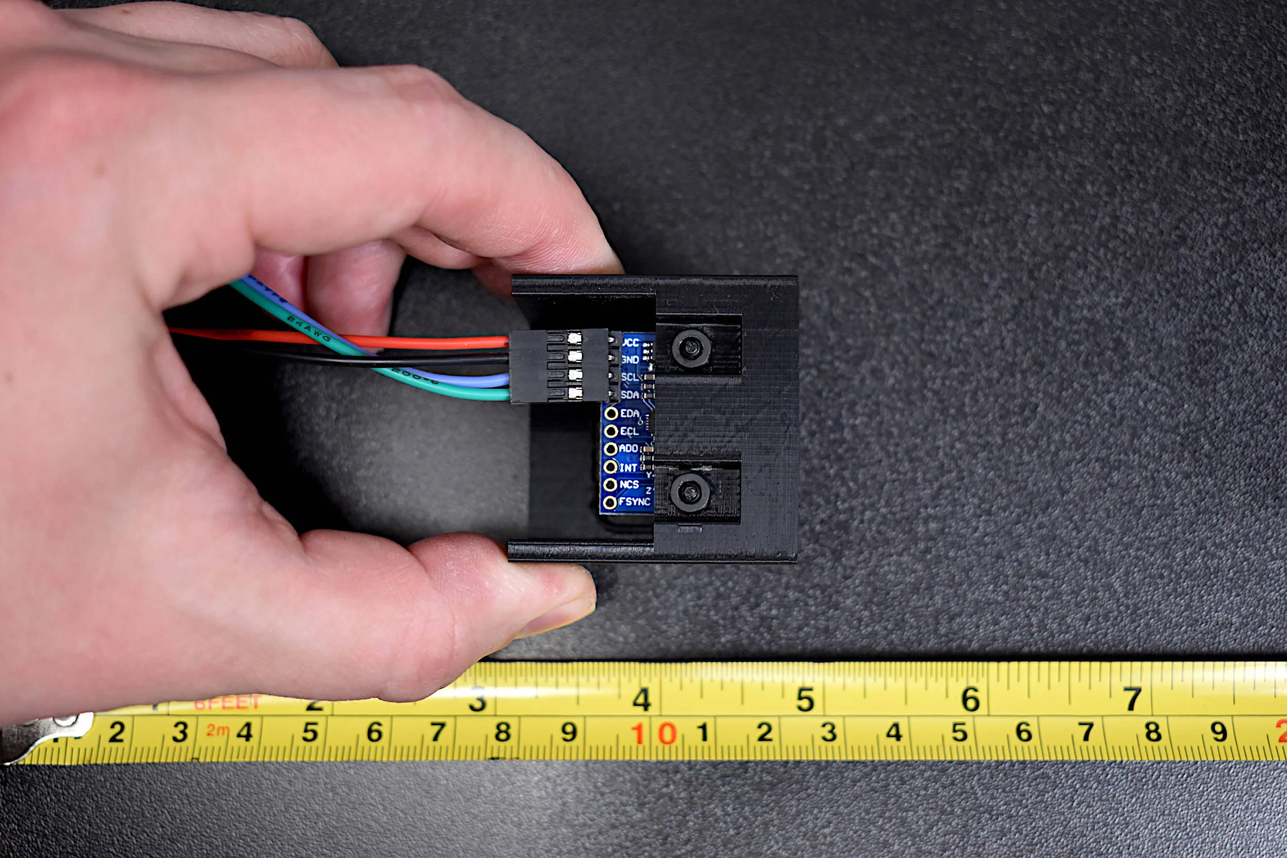
Returning to the MPU9250 magnetometer (AK8963) drawing, we can begin to understand how we might approximate the direction of magnetic north and the magnetic field strength at a the geographic location of the IMU:

Sensor Orientation of the MPU9250 (AK8963) Magnetometer
Similar to Part I of this tutorial series, we can use the magnetic field calculator produced by the National Centers for Environmental Information (NCEI) as a validation of the magnetic field being measured by the magnetometer. For New York City (our lab’s geographic location) the magnetic field components are as follows:

We can see that the magnetic field is being calculated by the World Magnetic Model 2010 for roughly downtown Manhattan, New York City. The declination is the angle between magnetic and geographic north. The inclination is the angle between the surface of the Earth and the vertical magnetic field. The horizontal intensity can be found by computing the amplitude of the component field in the horizontal direction. For example, if the IMU’s z-direction is placed parallel to gravity, the amplitude of the field in the x/y-directions can be found as follows:

The above can be used to find the strength of the magnetic field (horizontal intensity) using the two components of the field in the horizontal plane (x/y or any other combination depending on the orientation of the sensor). Similarly, we can approximate the heading using the arctangent of the two horizontal components as well:

Thus, using the arctangent relationship above the direction of magnetic north can be found using just two components of the magnetic field measured by the magnetometer (assuming the sensors are perpendicular to the surface). In the next section, the arctangent will be used to calibrate what is called the ‘hard iron offset’ for the magnetometer. This will effectively calibrate the offsets inherent in the magnetometer, and ensure that the angles being approximated from the arctangent are not biased by the sensors.
The IMU will need to be rotated 360 degrees in at least two directions in order to find the hard iron offset of the triple-axis magnetometer. The best way to understand hard iron effects is to first take measurements during a 360° rotation and visualize the magnetic response of the planar magnetometer sensors (sensors parallel to the Earth’s vertical magnetic field). This is shown in the plot below:

It is easy to see the large variability between the three sensor planes before offsetting for the hard iron effect. The 360° rotation of the sensor around each axis should produce a circle centered around the origin (0,0), which we see after offsetting for the hard iron effects. This is essential for improving the accuracy of the magnetometer’s approximation of heading. Thus, in the above we arrive at three offset values that approximate the hard iron interferences of the system. In the calculation of heading using the arctangent given in the above section, the hard iron effects should first be subtracted from the magnetometer values being read. This will increase the accuracy and stability of the tracking/orientation approximation being used for a given IMU application.
More information on hard iron offsets and magnetometer calibration can be found at the links below:
“Indoor Localization with Smartphones: Magnetometer Calibration” by Alwin Poulose
“Complete Triaxis Magnetometer Calibration in the Magnetic Domain” by Valérie Renaudin
The code used to conduct the hard iron calibration offset is also given below:
######################################################
# Copyright (c) 2021 Maker Portal LLC
# Author: Joshua Hrisko
######################################################
#
# This code reads data from the MPU9250/MPU9265 board
# (MPU6050 - accel/gyro, AK8963 - mag)
# and solves for tje hard iron offset for a
# magnetometer using a calibration block
#
#
######################################################
#
# wait 5-sec for IMU to connect
import time,sys
sys.path.append("../")
t0 = time.time()
start_bool = False # if IMU start fails - stop calibration
while time.time()-t0<5:
    try:
        from mpu9250_i2c import *
        start_bool = True
        break
    except:
        continue
import numpy as np
import csv,datetime
import matplotlib.pyplot as plt
from scipy.optimize import curve_fit

time.sleep(2) # wait for mpu to load
#
#####################################
# Mag Calibration Fitting
#####################################
#
def outlier_removal(x_ii,y_ii):
    x_diff = np.append(0.0,np.diff(x_ii)) # looking for outliers
    stdev_amt = 5.0 # standard deviation multiplier
    x_outliers = np.where(np.abs(x_diff)>np.abs(np.mean(x_diff))+\
                          (stdev_amt*np.std(x_diff)))
    x_inliers  = np.where(np.abs(x_diff)<np.abs(np.mean(x_diff))+\
                          (stdev_amt*np.std(x_diff)))
    y_diff     = np.append(0.0,np.diff(y_ii)) # looking for outliers
    y_outliers = np.where(np.abs(y_diff)>np.abs(np.mean(y_diff))+\
                          (stdev_amt*np.std(y_diff)))
    y_inliers  = np.abs(y_diff)<np.abs(np.mean(y_diff))+\
                 (stdev_amt*np.std(y_diff))
    if len(x_outliers)!=0:
        x_ii[x_outliers] = np.nan # null outlier
        y_ii[x_outliers] = np.nan # null outlier
    if len(y_outliers)!=0:
        y_ii[y_outliers] = np.nan # null outlier
        x_ii[y_outliers] = np.nan # null outlier
    return x_ii,y_ii

def mag_fit(x,a,b):
    return (a*x)+b

def mag_cal():
    print("-"*50)
    print("Magnetometer Calibration")
    mag_cal_rotation_vec = [] # variable for calibration calculations
    for qq,ax_qq in enumerate(mag_cal_axes):
        input("-"*8+" Press Enter and Start Rotating the IMU Around the "+ax_qq+"-axis")
        print("\t When Finished, Press CTRL+C")
        mag_array = []
        t0 = time.time()
        while True:
            try:
                mx,my,mz = AK8963_conv() # read and convert AK8963 magnetometer data
            except KeyboardInterrupt:
                break
            except:
                continue
            mag_array.append([mx,my,mz]) # mag array
        mag_array = mag_array[20:] # throw away first few points (buffer clearing)
        mag_cal_rotation_vec.append(mag_array) # calibration array
        print("Sample Rate: {0:2.0f} Hz".format(len(mag_array)/(time.time()-t0)))

    mag_cal_rotation_vec = np.array(mag_cal_rotation_vec) # make numpy array
    ak_fit_coeffs = []
    indices_to_save = [0,0,1] # indices to save as offsets
    for mag_ii,mags in enumerate(mag_cal_rotation_vec):
        mags = np.array(mags) # mag numpy array
        x,y = mags[:,cal_rot_indices[mag_ii][0]],\
                        mags[:,cal_rot_indices[mag_ii][1]] # sensors to analyze
        x,y = outlier_removal(x,y) # outlier removal
        y_0 = (np.nanmax(y)+np.nanmin(y))/2.0 # y-offset
        x_0 = (np.nanmax(x)+np.nanmin(x))/2.0 # x-offset
        ak_fit_coeffs.append([x_0,y_0][indices_to_save[mag_ii]]) # append to offset

    return ak_fit_coeffs,mag_cal_rotation_vec
#
#########################################
# Plot Values to See Calibration Impact
#########################################
#
def mag_cal_plot():
    plt.style.use('ggplot') # start figure
    fig,axs = plt.subplots(1,2,figsize=(12,7)) # start figure
    for mag_ii,mags in enumerate(mag_cal_rotation_vec):
        mags = np.array(mags) # magnetometer numpy array
        x,y = mags[:,cal_rot_indices[mag_ii][0]],\
                    mags[:,cal_rot_indices[mag_ii][1]]
        x,y = outlier_removal(x,y) # outlier removal
        axs[0].scatter(x,y,
                       label='Rotation Around ${0}$-axis (${1},{2}$)'.\
                    format(mag_cal_axes[mag_ii],
                           mag_labels[cal_rot_indices[mag_ii][0]],
                           mag_labels[cal_rot_indices[mag_ii][1]]))
        axs[1].scatter(x-mag_coeffs[cal_rot_indices[mag_ii][0]],
                    y-mag_coeffs[cal_rot_indices[mag_ii][1]],
                       label='Rotation Around ${0}$-axis (${1},{2}$)'.\
                    format(mag_cal_axes[mag_ii],
                           mag_labels[cal_rot_indices[mag_ii][0]],
                           mag_labels[cal_rot_indices[mag_ii][1]]))
    axs[0].set_title('Before Hard Iron Offset') # plot title
    axs[1].set_title('After Hard Iron Offset') # plot title
    mag_lims = [np.nanmin(np.nanmin(mag_cal_rotation_vec)),
                np.nanmax(np.nanmax(mag_cal_rotation_vec))] # array limits
    mag_lims = [-1.1*np.max(mag_lims),1.1*np.max(mag_lims)] # axes limits
    for jj in range(0,2):
        axs[jj].set_ylim(mag_lims) # set limits
        axs[jj].set_xlim(mag_lims) # set limits
        axs[jj].legend() # legend
        axs[jj].set_aspect('equal',adjustable='box') # square axes
    fig.savefig('mag_cal_hard_offset.png',dpi=300,bbox_inches='tight',
                facecolor='#FCFCFC') # save figure
    fig.savefig('mag_cal_hard_offset_white.png',dpi=300,bbox_inches='tight',
                facecolor='#FFFFFF') # save figure
    plt.show() #show plot

if __name__ == '__main__':
    if not start_bool:
        print("IMU not Started - Check Wiring and I2C")
    else:
        #
        ###################################
        # Magnetometer Calibration
        ###################################
        #
        mag_labels = ['m_x','m_y','m_z'] # mag labels for plots
        mag_cal_axes = ['z','y','x'] # axis order being rotated
        cal_rot_indices = [[0,1],[1,2],[0,2]] # indices of heading for each axis
        mag_coeffs,mag_cal_rotation_vec = mag_cal() # grab mag coefficients
        #
        ###################################
        # Plot with and without offsets
        ###################################
        #
        mag_cal_plot() # plot un-calibrated and calibrated results
        #
Once again, all codes are housed in the project repository at the link below:
The procedure for calibrating the hard offset for the magnetometer is as follows:
Run the mag_hard_calibration.py code (above)
When prompted, rotate the IMU around the stated axis (the stated axis should be parallel to gravity)
After rotating around the stated axis, press CTRL+C to interrupt the run
Repeat for all three axes
There is another more involved method for calibrating a magnetometer, called soft iron calibration, which scales each axis of the magnetometer to ensure that the shape of the rotation of the IMU maintains its circular form. If soft iron is present, the rotation of the IMU will produce more of an elliptic response rather than a circular one. This is not explored in this tutorial due to the lack of soft iron material present in our system. However, there are many publications that handle soft iron calibration for a magnetometer, below are just a few:
“Mitigation of magnetic interference and compensation of bias drift in inertial sensors” by Eric Christopher Frick
“Calibrating an eCompass in the Presence of Hard- and Soft-Iron Interference” by Talat Ozyagcilar
“Implementing a Tilt-Compensated eCompass using Accelerometer and Magnetometer Sensors” by Talat Ozyagcilar
In the next section, the fusion of all three sensors (9-degrees of freedom) will be introduced, which will combine all calibration routines that will output calibration coefficients in one script. Then, a live plotter will be given to permit real-time monitoring of all nine variables.

The calibration of the IMU has thus far only involved storing calibration coefficients in the local memory and producing plots and printouts of the variables. In this section, the calibration routines for each of the sensors is assembled into one calibration procedure where the coefficients are saved for future use. This makes the calibration procedure useful for future applications and allows for validation and extended verification of algorithms using the calibration information. This section will also introduce a real-time plotting code which allows the user to test the calibration of all 9-DoF in real time, which further validates the calibration and also helps users understand how the MPU9250 responds under different forcings (magnetic, accelerative, rotational, etc.).
The full calibration implementation code that goes through the calibration of the gyroscope, accelerometer, and magnetometer is given below. The code also outputs a real-time visualization for viewing the calibration of each 9-DoF along with an approximate heading calculation. The visualization allows for checking of calibration and verification of different phenomena in real-time. For example, a magnet could be brought into the IMU’s detection field and the response will be seen by the AK8963 magnetometer. The full code is given as well as on the project’s GitHub page.
######################################################
# Copyright (c) 2021 Maker Portal LLC
# Author: Joshua Hrisko
######################################################
#
# This code reads data from the MPU9250/MPU9265 board
# (MPU6050 - accel/gyro, AK8963 - mag)
# and solves for calibration coefficients for the
# accelerometer, gyroscope, and magnetometer using
# various methods with the IMU attached to a 3D-cube
# (MPU9250 + calibration block)
# --- The calibration coefficients are then saved to
# --- a local .csv file, which can be loaded upon
# --- the next run of the program
#
#
######################################################
#
# wait 5-sec for IMU to connect
import time
t0 = time.time()
start_bool = False # if IMU start fails - stop calibration
while time.time()-t0<5:
    try:
        from mpu9250_i2c import *
        start_bool = True
        break
    except:
        continue
import numpy as np
import csv,datetime
import matplotlib.pyplot as plt
from scipy.optimize import curve_fit

time.sleep(2) # wait for mpu to load
#
#####################################
# Gyro calibration (Steady)
#####################################
#
def gyro_cal():
    print("-"*50)
    print('Gyro Calibrating - Keep the IMU Steady')
    [mpu6050_conv() for ii in range(0,cal_size)] # clear buffer between readings
    mpu_array = [] # imu array for gyro vals
    gyro_offsets = [0.0,0.0,0.0] # gyro offset vector
    while True:
        try:
            _,_,_,wx,wy,wz = mpu6050_conv() # read and convert mpu6050 data
        except:
            continue

        mpu_array.append([wx,wy,wz]) # gyro vector append

        if np.shape(mpu_array)[0]==cal_size:
            for qq in range(0,3):
                gyro_offsets[qq] = np.mean(np.array(mpu_array)[:,qq]) # calc gyro offsets
            break
    print('Gyro Calibration Complete')
    return gyro_offsets # return gyro coeff offsets
#
#####################################
# Accel Calibration (gravity)
#####################################
#
def accel_fit(x_input,m_x,b):
    return (m_x*x_input)+b # fit equation for accel calibration
#
def get_accel():
    ax,ay,az,_,_,_ = mpu6050_conv() # read and convert accel data
    return ax,ay,az

def accel_cal():
    print("-"*50)
    print("Accelerometer Calibration")
    mpu_offsets = [[],[],[]] # offset array to be printed
    axis_vec = ['z','y','x'] # axis labels
    cal_directions = ["upward","downward","perpendicular to gravity"] # direction for IMU cal
    cal_indices = [2,1,0] # axis indices
    for qq,ax_qq in enumerate(axis_vec):
        ax_offsets = [[],[],[]]
        print("-"*50)
        for direc_ii,direc in enumerate(cal_directions):
            input("-"*8+" Press Enter and Keep IMU Steady to Calibrate the Accelerometer with the -"+\
              ax_qq+"-axis pointed "+direc)
            [mpu6050_conv() for ii in range(0,cal_size)] # clear buffer between readings
            mpu_array = []
            while len(mpu_array)<cal_size:
                try:
                    ax,ay,az = get_accel() # get accel variables
                    mpu_array.append([ax,ay,az]) # append to array
                except:
                    continue
            ax_offsets[direc_ii] = np.array(mpu_array)[:,cal_indices[qq]] # offsets for direction

        # Use three calibrations (+1g, -1g, 0g) for linear fit
        popts,_ = curve_fit(accel_fit,np.append(np.append(ax_offsets[0],
                                 ax_offsets[1]),ax_offsets[2]),
                   np.append(np.append(1.0*np.ones(np.shape(ax_offsets[0])),
                    -1.0*np.ones(np.shape(ax_offsets[1]))),
                        0.0*np.ones(np.shape(ax_offsets[2]))),
                            maxfev=10000)
        mpu_offsets[cal_indices[qq]] = popts # place slope and intercept in offset array
    print('Accelerometer Calibrations Complete')
    return mpu_offsets
#
#####################################
# Mag Calibration Fitting
#####################################
#
def outlier_removal(x_ii,y_ii):
    x_diff = np.append(0.0,np.diff(x_ii)) # looking for outliers
    stdev_amt = 5.0 # standard deviation multiplier
    x_outliers = np.where(np.abs(x_diff)>np.abs(np.mean(x_diff))+\
                          (stdev_amt*np.std(x_diff))) # outlier in x-var
    x_inliers  = np.where(np.abs(x_diff)<np.abs(np.mean(x_diff))+\
                          (stdev_amt*np.std(x_diff)))
    y_diff     = np.append(0.0,np.diff(y_ii)) # looking for outliers
    y_outliers = np.where(np.abs(y_diff)>np.abs(np.mean(y_diff))+\
                          (stdev_amt*np.std(y_diff))) # outlier in y-var
    y_inliers  = np.abs(y_diff)<np.abs(np.mean(y_diff))+\
                 (stdev_amt*np.std(y_diff)) # outlier vector
    if len(x_outliers)!=0:
        x_ii[x_outliers] = np.nan # null outlier
        y_ii[x_outliers] = np.nan # null outlier
    if len(y_outliers)!=0:
        y_ii[y_outliers] = np.nan # null outlier
        x_ii[y_outliers] = np.nan # null outlier
    return x_ii,y_ii

def mag_cal():
    print("-"*50)
    print("Magnetometer Calibration")
    cal_rot_indices = [[0,1],[1,2],[0,2]] # indices of heading for each axis
    mag_cal_rotation_vec = [] # variable for calibration calculations
    for qq,ax_qq in enumerate(mag_cal_axes):
        input("-"*8+" Press Enter and Start Rotating the IMU Around the "+ax_qq+"-axis")
        print("\t When Finished, Press CTRL+C")
        mag_array = []
        t0 = time.time()
        while True:
            try:
                mx,my,mz = AK8963_conv() # read and convert AK8963 magnetometer data
            except KeyboardInterrupt:
                break
            except:
                continue
            mag_array.append([mx,my,mz]) # mag array
        mag_array = mag_array[20:] # throw away first few points (buffer clearing)
        mag_cal_rotation_vec.append(mag_array) # calibration array
        print("Sample Rate: {0:2.0f} Hz".format(len(mag_array)/(time.time()-t0)))

    mag_cal_rotation_vec = np.array(mag_cal_rotation_vec) # make numpy array
    ak_fit_coeffs = [] # mag fit coefficient vector
    indices_to_save = [0,0,1] # indices to save as offsets
    for mag_ii,mags in enumerate(mag_cal_rotation_vec):
        mags = np.array(mags) # mag numpy array
        x,y = mags[:,cal_rot_indices[mag_ii][0]],\
                        mags[:,cal_rot_indices[mag_ii][1]] # sensors to analyze
        x,y = outlier_removal(x,y) # outlier removal
        y_0 = (np.nanmax(y)+np.nanmin(y))/2.0 # y-offset
        x_0 = (np.nanmax(x)+np.nanmin(x))/2.0 # x-offset
        ak_fit_coeffs.append([x_0,y_0][indices_to_save[mag_ii]]) # append to offset

    return ak_fit_coeffs
#
#####################################
# Plot Real-Time Values to Test
#####################################
#
def mpu_plot_test():
    #
    #############################
    # Figure/Axis Formatting
    #############################
    #
    plt.style.use('ggplot') # stylistic visualization
    fig = plt.figure(figsize=(12,9)) # start figure
    axs = [[],[],[],[]] # axis vector
    axs[0] = fig.add_subplot(321) # accel axis
    axs[1] = fig.add_subplot(323) # gyro axis
    axs[2] = fig.add_subplot(325) # mag axis
    axs[3] = fig.add_subplot(122,projection='polar') # heading axis
    plt_pts = 1000 # points to plot
    y_labels = ['Acceleration [g]','Angular Velocity [$^\circ/s$]','Magnetic Field [uT]']
    for ax_ii in range(0,len(y_labels)):
        axs[ax_ii].set_xlim([0,plt_pts]) # set x-limits for time-series plots
        axs[ax_ii].set_ylabel(y_labels[ax_ii]) # set y-labels
    ax_ylims = [[-4.0,4.0],[-300.0,300.0],[-100.0,100.0]] # ax limits
    for qp in range(0,len(ax_ylims)):
        axs[qp].set_ylim(ax_ylims[qp]) # set axis limits
    axs[3].set_rlim([0.0,100.0]) # set limits on heading plot
    axs[3].set_rlabel_position(112.5) # offset radius labels
    axs[3].set_theta_zero_location("N") # set north to top of plot
    axs[3].set_theta_direction(-1) # set rotation N->E->S->W
    axs[3].set_title('Magnetometer Heading') # polar plot title
    axs[0].set_title('Calibrated MPU9250 Time Series Plot') # imu time series title
    fig.canvas.draw() # draw axes
    #
    #############################
    # Pre-allocate plot vectors
    #############################
    #
    dummy_y_vals = np.zeros((plt_pts,)) # for populating the plots at start
    dummy_y_vals[dummy_y_vals==0] = np.nan # keep plots clear
    lines = [] # lines for looping updates
    for ii in range(0,9):
        if ii in range(0,3): # accel pre-allocation
            line_ii, = axs[0].plot(np.arange(0,plt_pts),dummy_y_vals,
                                label='$'+mpu_labels[ii]+'$',color=plt.cm.tab10(ii))
        elif ii in range(3,6): # gyro pre-allocation
            line_ii, = axs[1].plot(np.arange(0,plt_pts),dummy_y_vals,
                                label='$'+mpu_labels[ii]+'$',color=plt.cm.tab10(ii))
        elif ii in range(6,9): # mag pre-allocation
            jj = ii-6
            line_jj, = axs[2].plot(np.arange(0,plt_pts),dummy_y_vals,
                                label='$'+mpu_labels[ii]+'$',color=plt.cm.tab10(ii))
            line_ii, = axs[3].plot(dummy_y_vals,dummy_y_vals,
                                label='$'+mag_cal_axes[jj]+'$-Axis Heading',
                                   color=plt.cm.tab20b(int(jj*4)),
                                   linestyle='',marker='o',markersize=3)
            lines.append(line_jj)
        lines.append(line_ii)
    ax_legs = [axs[tt].legend() for tt in range(0,len(axs))] # legends for axes
    ax_bgnds = [fig.canvas.copy_from_bbox(axs[tt].bbox) for tt in range(0,len(axs))] # axis backgrounds
    fig.show() # show figure
    mpu_array = np.zeros((plt_pts,9)) # pre-allocate the 9-DoF vector
    mpu_array[mpu_array==0] = np.nan
    #
    #############################
    # Real-Time Plot Update Loop
    #############################
    #
    ii_iter = 0 # plot update iteration counter
    cal_rot_indicies = [[6,7],[7,8],[6,8]] # heading indices
    while True:
        try:
            ax,ay,az,wx,wy,wz = mpu6050_conv() # read and convert mpu6050 data
            mx,my,mz = AK8963_conv() # read and convert AK8963 magnetometer data
        except:
            continue

        mpu_array[0:-1] = mpu_array[1:] # get rid of last point
        mpu_array[-1] = [ax,ay,az,wx,wy,wz,mx,my,mz] # update last point w/new data

        if ii_iter==100:
            [fig.canvas.restore_region(ax_bgnds[tt]) for tt in range(0,len(ax_bgnds))] # restore backgrounds
            for ii in range(0,9):
                if ii in range(0,3):
                    lines[ii].set_ydata(cal_offsets[ii][0]*mpu_array[:,ii]+\
                                        cal_offsets[ii][1]) # update accel data array
                    axs[0].draw_artist(lines[ii]) # update accel plot
                if ii in range(3,6):
                    lines[ii].set_ydata(np.array(mpu_array[:,ii])-cal_offsets[ii]) # update gyro data
                    axs[1].draw_artist(lines[ii]) # update gyro plot
                if ii in range(6,9):
                    jj = ii-6 # index offsetted to 0-2
                    x = np.array(mpu_array[:,cal_rot_indicies[jj][0]]) # raw x-variable
                    y = np.array(mpu_array[:,cal_rot_indicies[jj][1]]) # raw y-variable
                    x_prime = x - cal_offsets[cal_rot_indicies[jj][0]] # x-var for heading
                    y_prime = y - cal_offsets[cal_rot_indicies[jj][1]] # y-var for heading
                    x_prime[np.isnan(x)] = np.nan
                    y_prime[np.isnan(y)] = np.nan
                    r_var = np.sqrt(np.power(x_prime,2.0)+np.power(y_prime,2.0)) # radius vector
                    theta = np.arctan2(-y_prime,x_prime) # angle vector for heading
                    lines[int(ii+jj)].set_ydata(mpu_array[:,ii]-\
                                            cal_offsets[cal_rot_indicies[jj][0]]) # update mag data
##                    lines[int(ii+jj+1)].set_data(x_prime,y_prime) # update heading data
                    lines[int(ii+jj+1)].set_data(theta,r_var)
                    axs[2].draw_artist(lines[int(ii+jj)]) # update mag plot
                    axs[3].draw_artist(lines[int(ii+jj+1)]) # update heading plot
            [axs[tt].draw_artist(ax_legs[tt]) for tt in range(0,len(ax_legs))] # update legends
            [fig.canvas.blit(axs[tt].bbox) for tt in range(0,len(ax_legs))] # update axes
            fig.canvas.flush_events() # flush blit events
            ii_iter = 0 # reset plot counter
        ii_iter+=1 # update plot counter

if __name__ == '__main__':
    if not start_bool:
        print("IMU not Started - Check Wiring and I2C")
    else:
        #
        ###################################
        # input parameters
        ###################################
        #
        mpu_labels = ['a_x','a_y','a_z','w_x','w_y','w_z','m_x','m_y','m_z']
        cal_labels = [['a_x','m','b'],['a_y','m','b'],['a_z','m','b'],'w_x','w_y','w_z',
                      ['m_x','m_x0'],['m_y','m_y0'],['m_z','m_z0']]
        mag_cal_axes = ['z','y','x'] # axis order being rotated for mag cal
        cal_filename = 'mpu9250_cal_params.csv' # filename for saving calib coeffs
        cal_size = 200 # how many points to use for calibration averages
        cal_offsets = np.array([[],[],[],0.0,0.0,0.0,[],[],[]]) # cal vector
        #
        ###################################
        # call to calibration functions
        ###################################
        #
        re_cal_bool = input("Input 1 + Press Enter to Calibrate New Coefficients or \n"+\
                            "Press Enter to Load Local Calibration Coefficients ")
        if re_cal_bool=="1":
            print("-"*50)
            input("Press Enter to Start The Calibration Procedure")
            time.sleep(1)
            gyro_offsets = gyro_cal() # calibrate gyro offsets under stable conditions
            cal_offsets[3:6] = gyro_offsets
            mpu_offsets = accel_cal() # calibrate accel offsets
            cal_offsets[0:3] = mpu_offsets
            ak_offsets = mag_cal() # calibrate mag offsets
            cal_offsets[6:] = ak_offsets
            # save calibration coefficients to file
            with open(cal_filename,'w',newline='') as csvfile:
                writer = csv.writer(csvfile,delimiter=',')
                for param_ii in range(0,len(cal_offsets)):
                    if param_ii>2:
                        writer.writerow([cal_labels[param_ii],cal_offsets[param_ii]])
                    else:
                        writer.writerow(cal_labels[param_ii]+
                                     [ii for ii in cal_offsets[param_ii]])
        else:
            # read calibration coefficients from file
            with open(cal_filename,'r',newline='') as csvfile:
                reader = csv.reader(csvfile,delimiter=',')
                iter_ii = 0
                for row in reader:
                    if len(row)>2:
                        row_vals = [float(ii) for ii in row[int((len(row)/2)+1):]]
                        cal_offsets[iter_ii] = row_vals
                    else:
                        cal_offsets[iter_ii] = float(row[1])
                    iter_ii+=1
        #
        ###################################
        # print out offsets for each sensor
        ###################################
        #
        print("-"*50)
        print('Offsets:')
        for param_ii,param in enumerate(cal_labels):
            print('\t{0}: {1}'.format(param,cal_offsets[param_ii]))
        print("-"*50)
        #
        ###################################
        # real-time plotter for validation
        ###################################
        #
        mpu_plot_test() # real-time plot of mpu calibratin verification
        #
An example printout of the calibration coefficients outputted by the script above can be seen below:

Calibration Coefficient Printout for the MPU9250
Another example output of the code above is given below showing a 360° rotation plot of the IMU around the z-axis:

The complete calibration code given above saves the calibration coefficients to a local file entitled 'mpu9250_cal_params.csv' - Upon reloading the parameters in this file, the calibration can be carried on into future applications.
This concludes the series entitled “Calibration of an Inertial Measurement Unit (IMU) with Raspberry Pi" (Part I, Part II) which outlined a series of measurement techniques desired around finding meaningful and useful calibration coefficients of an inertial measurement unit (IMU), specifically with an application employing the MPU9250 interfaced through a Raspberry Pi computer. The MPU9250 contains three sensors: an accelerometer, gyroscope (MPU6050), and magnetometer (AK8963), all of which were explored throughout the IMU calibration series. The accelerometer was calibrated using three data points for each axis, centered around Earth’s acceleration due to gravity. The gyroscope was calibrated under steady conditions to approximate the offset coefficients for each axis. In this entry, methods for calibrating the magnetometer were introduced, where the IMU was rotated 360° around each axis. Our IMU Calibration Block was used for all calibration procedures to permit calibration of all 9-degrees-of-freedom. Calibration of inertial measurement units is essential for improving algorithms deployed in applications ranging from autonomous vehicle navigation systems, gesture recognition, projectile guidance, indoor navigation, quadcopter navigation - just to name a few!

See More in Raspberry Pi and Engineering: