GOES-R Satellite Latitude and Longitude Grid Projection Algorithm

In this tutorial, I will discuss the methods used for calculation of latitude and longitude from a GOES-R L1b data file. The GOES-R L1b radiance files contain radiance data and geometry scan information in radians. This information is not enough to plot geographic radiance data right from the file, however, after some geometric manipulation harnessing satellite position and ellipsoid parameters, we can derive latitude and longitude values from the one-dimensional scan angles and plot our data in projected formats familiar to many geographic information tools.

Blog Post Index:

Theory: Satellite and Earth Geometry
Understanding Scan Angles (Radians)
Reprojecting Scan Angles (Radians) to Geographic Coordinates (Lat/Lon)
Exploring GOES-R netCDF Data Files
Algorithm Implementation: GOES-R Scan Angles (Radians) to Geographic Coordinates (Lat/Lon)
Visualizing GOES-R Data with The Derived Geographic Coordinate Grid Projection
Conclusion

Theory: Satellite And Earth Geometry

Satellite pixels can be approximated as an area on the surface of the earth. Each pixel can be identified by an angle at a certain height above Earth. The satellite produces angles in the x and y direction, while also giving us information about the height of the instrument and information about the earth. These parameters will allows us to approximate the latitude and longitude of each pixel after extrapolation onto the earth’s surface.

Each pixel needs information about the follow:

Geometry of the earth ellipsoid
Reference with respect to the earth’s center
Satellite properties from the point and center of Earth

Below is a depiction of the complex geometry involved in projecting the scan information from the satellite onto the earth’s geodetic coordinate system:

Based on the GOES-R product definition source (here, Page 20).

Now, we will derive the equations needed to go from the scan angles (in radians) to the latitude and longitude coordinates that we often associate with geographic information.

Understanding Scan Angles (Radians)

The GOES-R satellite produces netCDF4 data files that contain data and scan variables. The scan variables are called ‘x’ and ‘y’ GOES fixed grid projection coordinates in radians:

$\large x \equiv \textup{horizontal scan [radians]}$
$\large y \equiv \textup{vertical scan [radians]}$

The ‘x’ and ‘y’ projection coordinates merely give information about the angle of each pixel in reference to the imager. This looks like the following:

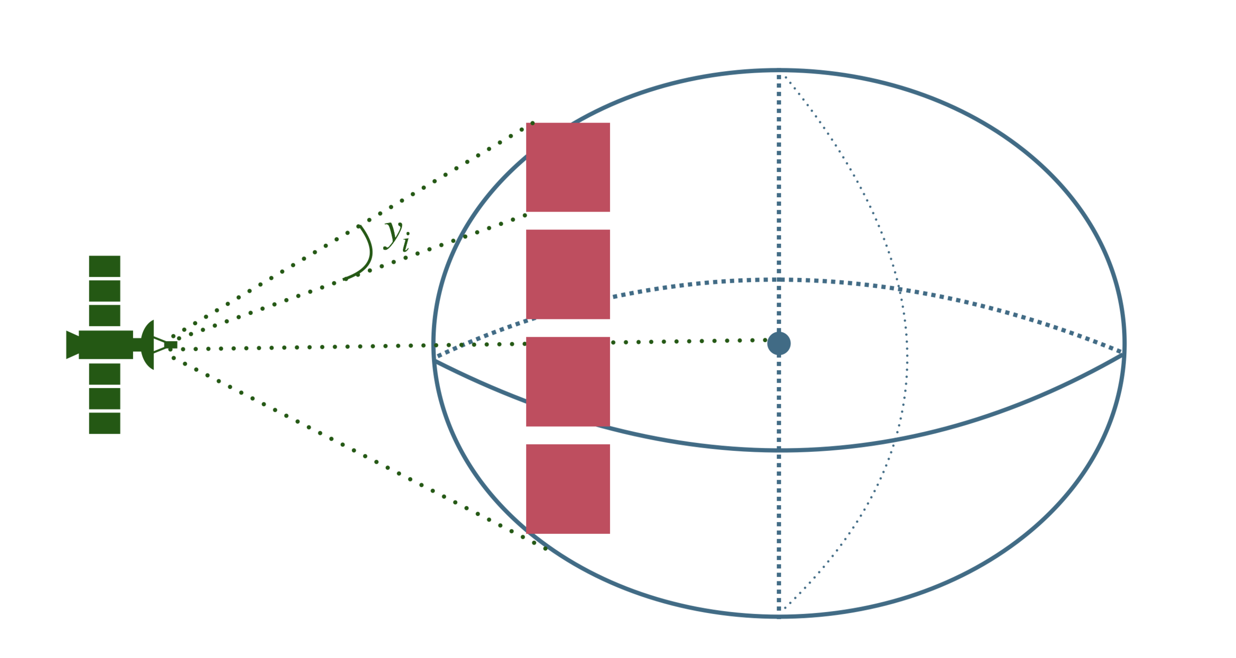
GOES-R exaggeration for visualizing scan angles in relation to the earth

Using the scan angles and the geometry above, we can derive the latitude and longitude grid to relate the data variables to ground-truth behavior. This method creates latitude and longitude arrays, which also aid in the calibration of satellite products, as well as integration with weather models based on geographic locations.

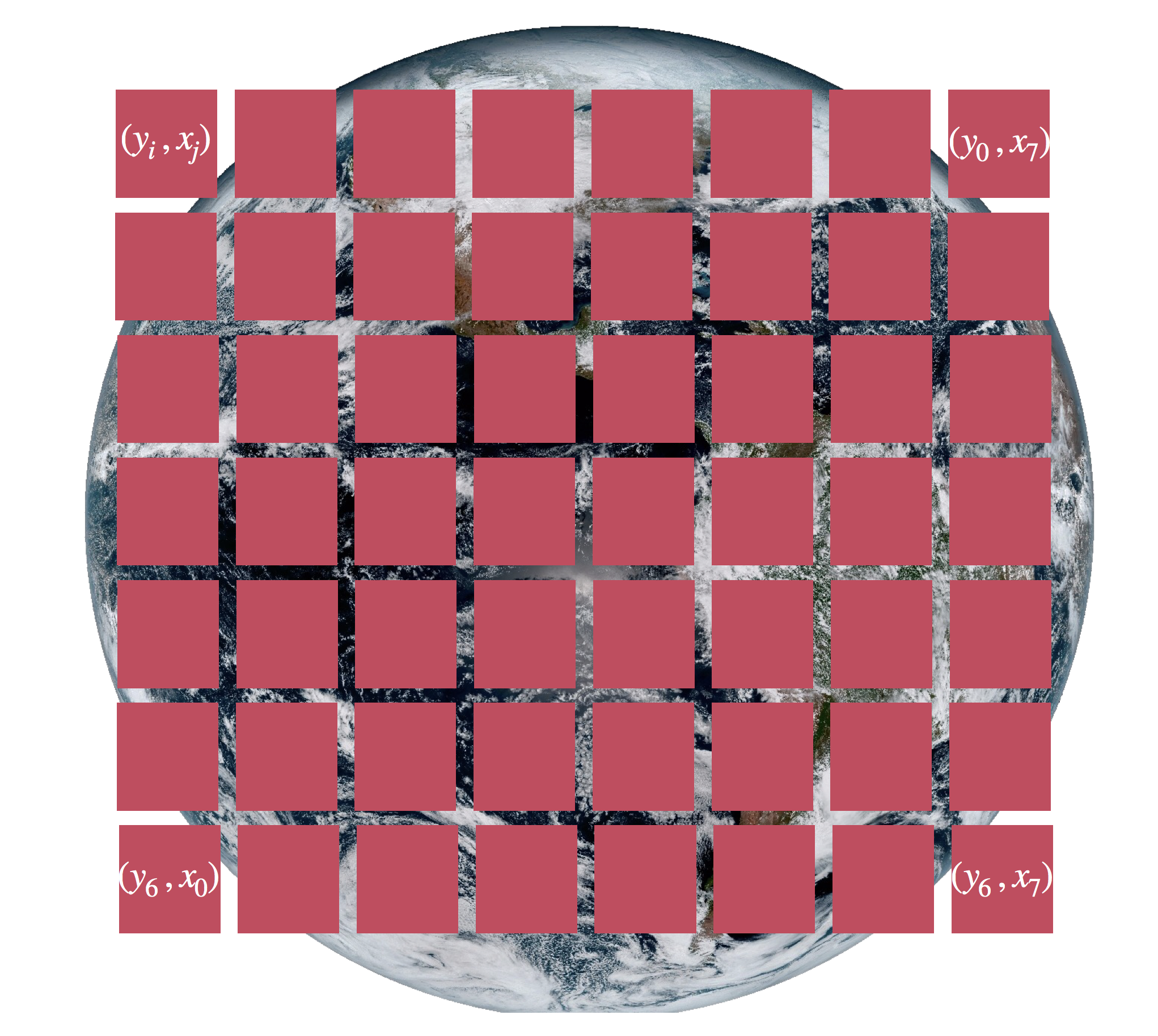
$\large x \, [\textup{radians}] \rightarrow \textup{latitude} \, [\textup{degrees}]$
$\large y \, [\textup{radians}] \rightarrow \textup{longitude} \, [\textup{degrees}]$

It is easy to think of the relationship above as one-to-one, but in reality, we need both scan angles to create latitude and longitude.

The scan angles can be gridded using the simple square array above, but then need to be converted using the complex geometry shown in the first figure above. In the next section, I outline the equations needed to transform the radian angles taken from the netCDF file and convert them to meaningful geographic latitude and longitude values. The reprojection will create a 2-D grid that we can then use to plot the data from each data file.

Reprojecting Scan Angles (Radians) to Geographic Coordinates (Lat/Lon)

Now that we have a rough understanding of satellite-earth geometry and the gridded scheme used in the GOES-R data files, we can introduce the complex series of equations used to reproject the scan angles down to the earth’s surface in terms of latitude and longitude coordinates.

From here, x represents the horizontal scan value at a given point, and y represents a vertical scan value at a given point. φ is the geodetic latitude of a corresponding point on the earth's surface, and λ is the geodetic longitude of the corresponding point. Below is the equation used to convert scan angles (x, y) to latitude and longitude (φ, λ):

$\large \phi = \arctan{\left( \frac{r_{eq}^2}{r_{pol}^2} \frac{s_z}{\sqrt{(H-s_x)^2 + s_y^2}}\right )}$
$\large \lambda = \lambda_0 - \arctan{\left( \frac{s_y}{H-s_x} \right )}$

where:

$\large r_{eq} = \textup{radius of Earth at the equator}$
$\large r_{pol} = \textup{radius of Earth at the pole}$
$\large H = \textup{distance from satellite to earth center}$
$\large \lambda_{0} = \textup{longitude of projection origin}$
$\large s_x ,\, s_y,\,s_z = \textup{derived using satellite location and earth geometry}$

I will not cover the derivation of each coordinate rotation (s_x,y,z) here, however, the methods can be found in nearly any orbital mechanics textbook. The coordinate rotations are defined as follows:

$\large s_x = r_s \cos{(x)}\cos{(y)}$
$\large s_y = -r_s \sin{(x)}$
$\large s_z = r_s \cos{(x)}\sin{(y)}$

Again, the x, y are the scan angles given by the netCDF data file. From here, we further define:

$\large r_s = \frac{-b - \sqrt{b^2 - 4ac}}{2a}$

Which was found using the quadratic equation and the geometry above. The variables are defined as:

$\large a = \sin^2{x} + \cos^2{x} \left(\cos^2{y} + \frac{r_{eq}^2}{r_{pol}^2} \sin^2{y}\right )$
$\large b = -2H\cos{(x)}\cos{(y)}$
$\large c = H^2 - r_{eq}^2$

And now we’re ready to calculate our latitude and longitude grid from the information give to us by the GOES-R satellite data files.

$\large \phi \, [\textup{latitude}]= \arctan{\left( \frac{r_{eq}^2}{r_{pol}^2} \frac{s_z}{\sqrt{(H-s_x)^2 + s_y^2}}\right )}$
$\large \lambda \, [\textup{longitude}]= \lambda_0 - \arctan{\left( \frac{s_y}{H-s_x} \right )}$

Exploring GOES-R netCDF Data Files

The GOES-R files contain information needed to use the equations above. GOES-R data can be found on the Google Cloud server located here:

https://console.cloud.google.com/storage/browser/gcp-public-data-goes-16

Download a test file from one of the folders (I recommend using ‘gcp-public-data-goes-16/ABI-L1b-RadC/2018’ which is recent raw radiance data from 2018. Once the file is downloaded and put into a nearby directory (I put mine into ‘./rad_nc_files/’) we can start analzing the .nc file.

The following code reads a netCDF file and creates a projection variables called ‘proj_info’ which contains many of the variables needed in the equations above:

#!/usr/bin/python

from netCDF4 import Dataset
import os

# navigate to directory with .nc data files (raw radiance files in my case)
os.chdir('./rad_nc_files/')
full_direc = os.listdir()
nc_files = [ii for ii in full_direc if ii.endswith('.nc')]
nc_indx = 5 
g16_data_file = nc_files[nc_indx] # select .nc file
print(nc_files[nc_indx]) # print file name

# designate dataset
g16nc = Dataset(g16_data_file, 'r')

# GOES-R projection info
proj_info = g16nc.variables['goes_imager_projection']

Printing out the ‘proj_info’ variable yields the following:

<class 'netCDF4._netCDF4.Variable'>
  int32 goes_imager_projection()
  long_name: GOES-R ABI fixed grid projection
  grid_mapping_name: geostationary
  perspective_point_height: 35786023.0
  semi_major_axis: 6378137.0
  semi_minor_axis: 6356752.31414
  inverse_flattening: 298.2572221
  latitude_of_projection_origin: 0.0
  longitude_of_projection_origin: -75.0
  sweep_angle_axis: x
  unlimited dimensions: 
  current shape = ()
  filling on, default _FillValue of -2147483647 used

There are several very important variables to be taken from this list:

$\large r_{eq} = \textup{semi\_major\_axis: 6378137.0}$
$\large r_{pol} = \textup{semi\_minor\_axis: 6356752.31414}$
$\large \lambda_0 = \textup{longitude\_of\_projection\_origin: -75.0}$
$\large h_{sat} = \textup{perspective\_point\_height: 35786023.0}$
$\large H = r_{eq} + h_{sat} = 42164160.0$

With the variables above, we now have enough information to go from the data files that contain 1-D radian angles to latitude and longitude grids. In the next section I will introduce the actual algorithm for calculating lat/lon grids from radian angles.

Algorithm Implementation: GOES-R Scan Angles (Radians) to Geographic Coordinates (Lat/Lon)

Now that all the groundwork has been built, we can calculate the actual grid for a given netCDF data file. The Python program is introduced below:

#!/usr/bin/python

from netCDF4 import Dataset
import numpy as np
import os

# navigate to directory with .nc data files (raw radiance files in my case)
os.chdir('./rad_nc_files/')
full_direc = os.listdir()
nc_files = [ii for ii in full_direc if ii.endswith('.nc')]
nc_indx = 5
g16_data_file = nc_files[nc_indx] # select .nc file
print(nc_files[nc_indx]) # print file name

# designate dataset
g16nc = Dataset(g16_data_file, 'r')

# GOES-R projection info and retrieving relevant constants
proj_info = g16nc.variables['goes_imager_projection']
lon_origin = proj_info.longitude_of_projection_origin
H = proj_info.perspective_point_height+proj_info.semi_major_axis
r_eq = proj_info.semi_major_axis
r_pol = proj_info.semi_minor_axis

# Data info
lat_rad_1d = g16nc.variables['x'][:]
lon_rad_1d = g16nc.variables['y'][:]

# close file when finished
g16nc.close()
g16nc = None

# create meshgrid filled with radian angles
lat_rad,lon_rad = np.meshgrid(lat_rad_1d,lon_rad_1d)

# lat/lon calc routine from satellite radian angle vectors

lambda_0 = (lon_origin*np.pi)/180.0

a_var = np.power(np.sin(lat_rad),2.0) + (np.power(np.cos(lat_rad),2.0)*(np.power(np.cos(lon_rad),2.0)+(((r_eq*r_eq)/(r_pol*r_pol))*np.power(np.sin(lon_rad),2.0))))
b_var = -2.0*H*np.cos(lat_rad)*np.cos(lon_rad)
c_var = (H**2.0)-(r_eq**2.0)

r_s = (-1.0*b_var - np.sqrt((b_var**2)-(4.0*a_var*c_var)))/(2.0*a_var)

s_x = r_s*np.cos(lat_rad)*np.cos(lon_rad)
s_y = - r_s*np.sin(lat_rad)
s_z = r_s*np.cos(lat_rad)*np.sin(lon_rad)

lat = (180.0/np.pi)*(np.arctan(((r_eq*r_eq)/(r_pol*r_pol))*((s_z/np.sqrt(((H-s_x)*(H-s_x))+(s_y*s_y))))))
lon = (lambda_0 - np.arctan(s_y/(H-s_x)))*(180.0/np.pi)


# print test coordinates
print('{} N, {} W'.format(lat[318,1849],abs(lon[318,1849])))

If your algorithm is correct and your data file is 1500 x 2500, then your output above should look like the following:

Screen Shot 2018-11-25 at 5.49.31 PM.png

The screenshot above tells the user a few things:

The name of the netCDF file read in
There were negative values under the square root in the calculation of r_s
There were negative values under the square root in the calculation of latitude
The values for latitude and longitude at a specific point were successful

If your screenshot looks similar to the one above - CONGRATULATIONS. The code worked. The values outputted by the program are the latitude and longitude of the pixel nearest to New York City. Now, you have a grid for latitude and longitude that is the same size as the data array in the netCDF file. In the next section we will use this to plot and visualize the data!

Coordinates for nearest pixel to New York City aboard the GOES-R satellite

Visualizing GOES-R Data with The Derived Geographic Coordinate Grid Projection

Below is a simple implementation of the grid projection algorithm above, which takes the grid and projects the data onto a basemap using Python’s Basemap Toolkit.

#!/usr/bin/python

from netCDF4 import Dataset
import matplotlib as mpl
mpl.use('TkAgg')
import matplotlib.pyplot as plt
from mpl_toolkits.basemap import Basemap, cm
import numpy as np
import os

def lat_lon_reproj(nc_folder,nc_indx):
    os.chdir(nc_folder)
    full_direc = os.listdir()
    nc_files = [ii for ii in full_direc if ii.endswith('.nc')]
    g16_data_file = nc_files[nc_indx] # select .nc file
    print(nc_files[nc_indx]) # print file name

    # designate dataset
    g16nc = Dataset(g16_data_file, 'r')
    var_names = [ii for ii in g16nc.variables]
    var_name = var_names[0]
    try:
        band_id = g16nc.variables['band_id'][:]
        band_id = ' (Band: {},'.format(band_id[0])
        band_wavelength = g16nc.variables['band_wavelength']
        band_wavelength_units = band_wavelength.units
        band_wavelength_units = '{})'.format(band_wavelength_units)
        band_wavelength = ' {0:.2f} '.format(band_wavelength[:][0])
        print('Band ID: {}'.format(band_id))
        print('Band Wavelength: {} {}'.format(band_wavelength,band_wavelength_units))
    except:
        band_id = ''
        band_wavelength = ''
        band_wavelength_units = ''

    # GOES-R projection info and retrieving relevant constants
    proj_info = g16nc.variables['goes_imager_projection']
    lon_origin = proj_info.longitude_of_projection_origin
    H = proj_info.perspective_point_height+proj_info.semi_major_axis
    r_eq = proj_info.semi_major_axis
    r_pol = proj_info.semi_minor_axis

    # grid info
    lat_rad_1d = g16nc.variables['x'][:]
    lon_rad_1d = g16nc.variables['y'][:]

    # data info    
    data = g16nc.variables[var_name][:]
    data_units = g16nc.variables[var_name].units
    data_time_grab = ((g16nc.time_coverage_end).replace('T',' ')).replace('Z','')
    data_long_name = g16nc.variables[var_name].long_name
    
    # close file when finished
    g16nc.close()
    g16nc = None

    # create meshgrid filled with radian angles
    lat_rad,lon_rad = np.meshgrid(lat_rad_1d,lon_rad_1d)

    # lat/lon calc routine from satellite radian angle vectors

    lambda_0 = (lon_origin*np.pi)/180.0

    a_var = np.power(np.sin(lat_rad),2.0) + (np.power(np.cos(lat_rad),2.0)*(np.power(np.cos(lon_rad),2.0)+(((r_eq*r_eq)/(r_pol*r_pol))*np.power(np.sin(lon_rad),2.0))))
    b_var = -2.0*H*np.cos(lat_rad)*np.cos(lon_rad)
    c_var = (H**2.0)-(r_eq**2.0)

    r_s = (-1.0*b_var - np.sqrt((b_var**2)-(4.0*a_var*c_var)))/(2.0*a_var)

    s_x = r_s*np.cos(lat_rad)*np.cos(lon_rad)
    s_y = - r_s*np.sin(lat_rad)
    s_z = r_s*np.cos(lat_rad)*np.sin(lon_rad)

    lat = (180.0/np.pi)*(np.arctan(((r_eq*r_eq)/(r_pol*r_pol))*((s_z/np.sqrt(((H-s_x)*(H-s_x))+(s_y*s_y))))))
    lon = (lambda_0 - np.arctan(s_y/(H-s_x)))*(180.0/np.pi)


    # print test coordinates
    print('{} N, {} W'.format(lat[318,1849],abs(lon[318,1849])))

    return lon,lat,data,data_units,data_time_grab,data_long_name,band_id,band_wavelength,band_wavelength_units,var_name

nc_folder = './rad_nc_files/' # define folder where .nc files are located

file_indx = 15 # be sure to pick the correct file. Make sure the file is not too big either,
# some of the bands create large files (stick to band 7-16)

# main data grab from function above
lon,lat,data,data_units,data_time_grab,data_long_name,band_id,band_wavelength,band_units,var_name = lat_lon_reproj(nc_folder,file_indx)

bbox = [np.min(lon),np.min(lat),np.max(lon),np.max(lat)] # set bounds for plotting

# figure routine for visualization
fig = plt.figure(figsize=(9,4),dpi=200)

n_add = 0
m = Basemap(llcrnrlon=bbox[0]-n_add,llcrnrlat=bbox[1]-n_add,urcrnrlon=bbox[2]+n_add,urcrnrlat=bbox[3]+n_add,resolution='i', projection='cyl')
m.drawcoastlines(linewidth=0.5)
m.drawcountries(linewidth=0.25)
m.pcolormesh(lon.data, lat.data, data, latlon=True)
parallels = np.linspace(np.min(lat),np.max(lat),5.)
m.drawparallels(parallels,labels=[True,False,False,False])
meridians = np.linspace(np.min(lon),np.max(lon),5.)
m.drawmeridians(meridians,labels=[False,False,False,True])
cb = m.colorbar()

data_units = ((data_units.replace('-','^{-')).replace('1','1}')).replace('2','2}')
plt.rc('text', usetex=True)
cb.set_label(r'%s $ \left[ \mathrm{%s} \right] $'% (var_name,data_units))
plt.title('{0}{2}{3}{4} on {1}'.format(data_long_name,data_time_grab,band_id,band_wavelength,band_units))
plt.tight_layout()

#plt.savefig('goes_16_demo.png',dpi=200,transparent=True) # uncomment to save figure
plt.show()

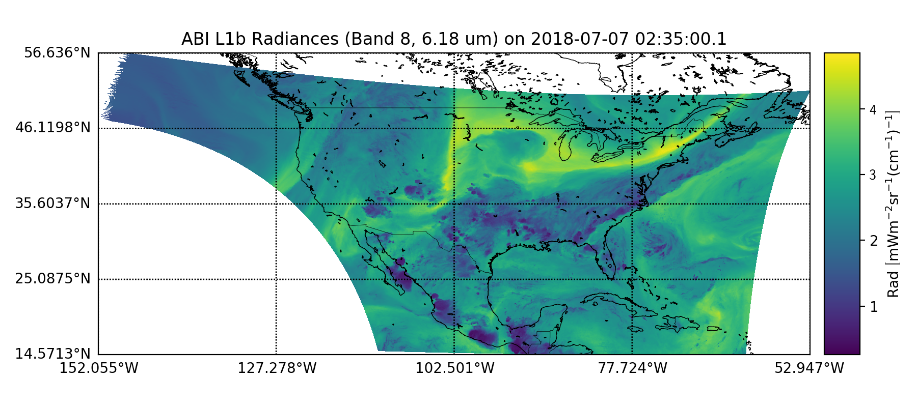
If analyzing raw radiance data, the figure below is the expected output. It has information about the data (ABI L1b Radiances), the band ID (8th band, the band wavelength (6.118 microns), and the date (July 7th, 2018).

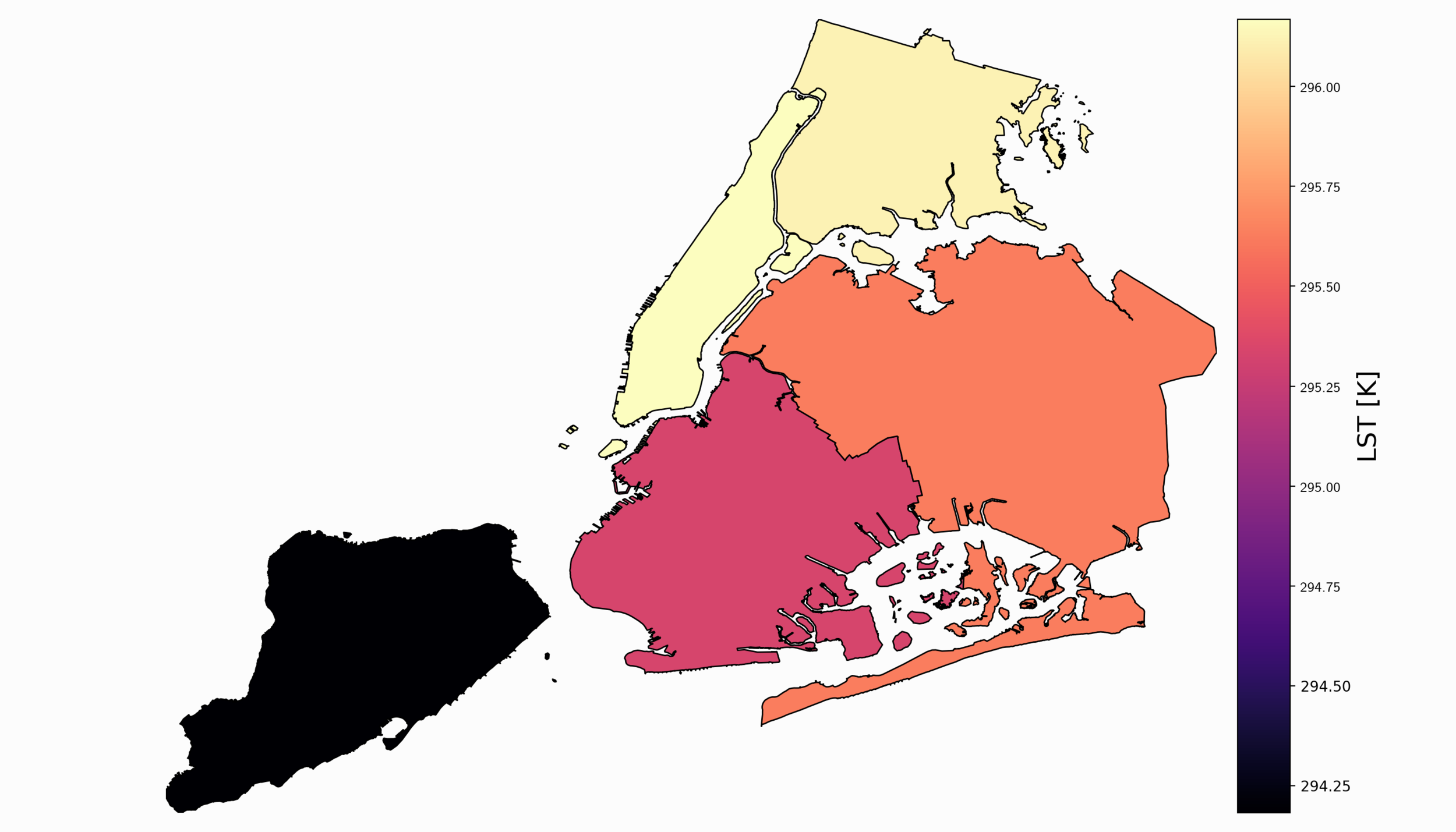
GOES-R ABI L1b Radiance Plot Example.png

In contrast to the figure above, the figure below is taken from the GOES-R processed land surface temperature (LST) product. The LST product is used for applications in weather modeling and prediction, real-time information on fires and other natural hazards, historical behavior in relation to crops, and much more. A snapshot taken from the 6th of June, 2018 is shown below:

Land Surface Temperature from GOES-R Satellite Example.png

Notice how the figure directly above masks the off-land data. This is how many algorithms handle product data - they filter out data that may be over water, typically using some sort of elevation mask. There are also other masks that filter cloudy data and other low quality data that may have interference between the satellite and the surface of the earth.

Conclusion

This concludes the tutorial on creating latitude and longitude grids from netCDF files that only contain 1-dimensional scan angles. This is a great practice in understanding satellites and orbital mechanics. In the tutorial I covered some basics on orbiting satellites and scanning methods used by satellites. While I didn’t derive the complex geometric equations, I demonstrated how to use them and implement the algorithms used for plotting satellite imagery in Python. Python was able to handle reading and plotting of data fairly quickly, which makes this a powerful method for plotting satellite imagery. One may want to create a grid file and save it, so that the algorithm can be sped up when reading geostationary satellite imagery. However, for an introduction into orbiting satellites and reading netCDF data, while visualizing imagery, it’s a great foray into visualizing radiances from satellites.

See More in Engineering and GIS:

Featured