Satellite Imagery Analysis in Python Part III: Land Surface Temperature and The National Land Cover Database (NLCD)

This is the third entry in the satellite imagery analysis in Python series. For part I, click here, for part II, click here.
In this tutorial we will use land surface temperature (LST) as the data variable along with land cover information from the national (U.S.) database. The land cover information will allow us to create a relationship between land cover type and its respective heating (or cooling) contribution to the earth’s surface. Land cover is used in many applications ranging from algorithm development to military applications and crop surveying, not to mention applications in water management and drought awareness.
The Multi-Resolution Land Characteristics (MRLC) consortium produces the National Land Cover Database (NLCD) for the U.S. at 30-m resolution. The database defines 16 land cover classes for the lower 48 states (there are 4 more specifically for Alaska that we won’t use) that range from water, urbanization, forestation, and more. The NLCD from 2016 (the most recent version) can be downloaded from the following link:
https://s3-us-west-2.amazonaws.com/mrlc/NLCD_2016_Land_Cover_L48_20190424.zip
The file is quite large (1.4GB compressed and zipped). I recommend pulling the NLCD data into a GIS software and clipping the bounds to the particular area of interested (i.e. New York City in our case) - this will allow us to minimize the amount of processing needed between Python and the NLCD data.
In Python, the NLCD raster file needs to be read in using a geo toolbox. I chose to use rasterio because it is more familiar to me, however, other libraries are capable of handling the reading of the raster. The full methodology behind handling and plotting the NLCD raster file is quite involved and could be an entire tutorial, however, I will leave much of the explanation in the comments of the Python code. The breakdown for reading the NLCD is briefly explained below:
First, we read in the city boundary (NYC in this case) and set the bounding latitude and longitude points
Read the NLCD raster file to get its affine transform information - we will use this to inverse the NYC lat/lon boundaries to find the endpoints in raster file coordinates
Create a meshgrid for latitude and longitude in raster coordinates
Transform meshgrid to WGS84 coordinates using affine transform
Read NLCD data using lat/lon boundary indices
Read and delineate colors for NLCD bands
Map NLCD data
The full code for plotting NYC’s NLCD map is shown below, along with the corresponding figure output:
import matplotlib as mpl
mpl.use('TkAgg')
import matplotlib.pyplot as plt
from matplotlib.colors import ListedColormap
from mpl_toolkits.basemap import Basemap
import numpy as np
from osgeo import gdal,ogr,osr
import os,pyproj,rasterio

# function for calculating NLCD values in plot window
def format_coord(x, y):
    indx = np.argmin(np.abs(np.subtract(x,lons))+np.abs(np.subtract(y,lats)))
    indx = np.unravel_index(indx,np.shape(lats))
    z = nlcd[indx]
    z_str = leg_str[int(np.where(z==legend)[0])]
    return f', , NLCD:  ()'

# legend indices and strings that represent each land cover type
legend = np.array([0,11,12,21,22,23,24,31,41,42,43,51,52,71,72,73,74,81,82,90,95])
leg_str = np.array(['NaN','Open Water','Perennial Ice/Snow','Developed, Open Space','Developed, Low Intensity',
           'Developed, Medium Intensity','Developed High Intensity','Barren Land (Rock/Sand/Clay)',
           'Deciduous Forest','Evergreen Forest','Mixed Forest','Dwarf Scrub','Shrub/Scrub',
           'Grassland/Herbaceous','Sedge/Herbaceous','Lichens','Moss','Pasture/Hay','Cultivated Crops',
           'Woody Wetlands','Emergent Herbaceous Wetlands'])

# reading NYC shapefile to set boundaries
shapefile_folder = './Borough Boundaries/'
shapefile_name = 'geo_export_ade24428-c163-42c7-9e6d-7e9743323143'
drv    = ogr.GetDriverByName('ESRI Shapefile') # define shapefile driver
ds_in  = drv.Open(shapefile_folder+shapefile_name+'.shp',0) #open shapefile
lyr_in = ds_in.GetLayer() # grab layer
sourceprj = (lyr_in.GetSpatialRef()) # input projection
targetprj = osr.SpatialReference()
targetprj.ImportFromEPSG(4326) # wanted projection
transform = osr.CoordinateTransformation(sourceprj, targetprj)
shp = lyr_in.GetExtent()
ll_x,ll_y,_ = transform.TransformPoint(shp[0],shp[2]) # reprojected bounds for city
ur_x,ur_y,_ = transform.TransformPoint(shp[1],shp[3]) # reprojected bounds for city
bbox = [ll_x,ll_y,ur_x,ur_y] # bounding box

# reproject shapefile (if correct projection, the same is return; if incorrect
# it will reproject to WGS84)
outputShapefile = shapefile_folder+shapefile_name+'_correct_CRS.shp'
if os.path.exists(outputShapefile):
    drv.DeleteDataSource(outputShapefile)
outDataSet = drv.CreateDataSource(outputShapefile)
outLayer = outDataSet.CreateLayer("correct_CRS", geom_type=ogr.wkbMultiPolygon)

# add fields
inLayerDefn = lyr_in.GetLayerDefn()
for i in range(0, inLayerDefn.GetFieldCount()):
    fieldDefn = inLayerDefn.GetFieldDefn(i)
    outLayer.CreateField(fieldDefn)

# get the output layer's feature definition
outLayerDefn = outLayer.GetLayerDefn()

inFeature = lyr_in.GetNextFeature()
while inFeature:
    # get the input geometry
    geom = inFeature.GetGeometryRef()
    # reproject the geometry
    geom.Transform(transform)
    # create a new feature
    outFeature = ogr.Feature(outLayerDefn)
    # set the geometry and attribute
    outFeature.SetGeometry(geom)
    for i in range(0, outLayerDefn.GetFieldCount()):
        outFeature.SetField(outLayerDefn.GetFieldDefn(i).GetNameRef(), inFeature.GetField(i))
    # add the feature to the shapefile
    outLayer.CreateFeature(outFeature)
    # dereference the features and get the next input feature
    outFeature = None
    inFeature = lyr_in.GetNextFeature()
    # Save and close the shapefiles
inDataSet = None
outDataSet = None

# NLCD folder
cwd = os.getcwd() # change to NLCD folder
nlcd_filename = 'NLCD_2016_Land_Cover_L48_20190424.img' # NLCD raster
os.chdir('./NLCD_2016_Land_Cover_L48_20190424/') # location of NLCD raster

# routine for computing affine transformation for projection of lat/lon eastings
with rasterio.open(nlcd_filename) as r:
    T0 = r.transform

inproj = pyproj.Proj(init='epsg:4326') # NYC bbox projection
outproj = pyproj.Proj('+proj=aea +lat_1=29.5 +lat_2=45.5 +lat_0=23.0 '+\
                      '+lon_0=-96 +x_0=0 +y_0=0 +datum=NAD83 +towgs84=0,0,0,0 +units=m +no_defs') # NLCD proj.

# inversing bounding box coordinates to NLCD local coordinate system indices
x_ll,y_ll = ~T0*((pyproj.transform(inproj,outproj,bbox[0],bbox[1])))
x_ul,y_ul = ~T0*((pyproj.transform(inproj,outproj,bbox[0],bbox[3])))
x_lr,y_lr = ~T0*((pyproj.transform(inproj,outproj,bbox[2],bbox[1])))
x_ur,y_ur = ~T0*((pyproj.transform(inproj,outproj,bbox[2],bbox[3])))
x_span = [x_ll,x_ul,x_lr,x_ur]
y_span = [y_ll,y_ul,y_lr,y_ur]

# calculating NLCD image bounds that relate to NYC bbox
cols, rows = np.meshgrid(np.arange(r.width)[int(np.min(x_span)):int(np.max(x_span))],
                       np.arange(r.height)[int(np.min(y_span)):int(np.max(y_span))])
eastings,northings = (cols,rows)*T0

# transformation from raw projection to WGS84 lat/lon values
inproj = pyproj.Proj('+proj=aea +lat_1=29.5 +lat_2=45.5 +lat_0=23.0 +lon_0=-96 +x_0=0 +y_0=0'+\
                     ' +datum=NAD83 +towgs84=0,0,0,0 +units=m +no_defs')
outproj = pyproj.Proj(init='epsg:4326')
xvals,yvals = (eastings,northings)
lons,lats = (pyproj.transform(inproj,outproj,xvals,yvals)) # actual lats/lons

# reading NLCD data from bounds
ds = gdal.Open(nlcd_filename)
nlcd_reader = ds.GetRasterBand(1)
nlcd = nlcd_reader.ReadAsArray(int(np.min(x_span)),int(np.min(y_span)),
                               int(np.max(x_span))-int(np.min(x_span)),int(np.max(y_span))-int(np.min(y_span)))

# colormap determination and setting bounds
with rasterio.open(nlcd_filename) as r:
    cmap_in = r.colormap(1)
    cmap1 = [[np.int(jj) for jj in cmap_in[ii]] for ii in cmap_in]
    cmap_in = [[np.float(jj)/255.0 for jj in cmap_in[ii]] for ii in cmap_in]
    indx_list = np.unique(nlcd)
    r_cmap = []
    for ii in indx_list:
        r_cmap.append(cmap_in[ii])
    raster_cmap = ListedColormap(r_cmap) # defining the NLCD specific color map
    norm = mpl.colors.BoundaryNorm(indx_list, raster_cmap.N) # specifying colors based on num. unique points

# plot NLCD
os.chdir(cwd) # change directory back
fig,ax = plt.subplots(figsize=(14,9))
m = Basemap(llcrnrlon=bbox[0],llcrnrlat=bbox[1],urcrnrlon=bbox[2],
            urcrnrlat=bbox[3],resolution='i', projection='cyl')
m.readshapefile(shapefile_folder+shapefile_name+'_correct_CRS','city_shapefile')
parallels = np.linspace(bbox[1],bbox[3],5.) # latitudes
m.drawparallels(parallels,labels=[True,False,False,False],fontsize=12)
meridians = np.linspace(bbox[0],bbox[2],5.) # longitudes
m.drawmeridians(meridians,labels=[False,False,False,True],fontsize=12)
m.pcolormesh(lons,lats,nlcd, latlon=True,norm=norm,
             alpha=0.9,cmap=raster_cmap) # plotting actual LST data
ax.format_coord = format_coord # update cursor function
ax.set_xlabel(' ')
ax.set_ylabel(' ')
fig.tight_layout()
##plt.savefig('nlcd_mapper_colors_EL_PASO.png',dpi=150,facecolor=[252/255,252/255,252/255])
plt.show()
Above, we see that New York City is highly urban!
Below is a similar map of El Paso, TX. We can see the vast difference in land cover across the two cities. New York is highly urban, and while El Paso is urban as well, much of the outlying area is shrubbery and herbaceous desert-like land covers.
NLCD for El Paso, TX

Beneath El Paso, there is a region of darkness, which simply represents the change from the U.S. to Mexico. And since this is a U.S. land cover product, we do not have any data in that region. I’ve included a third NLCD map for the city of Phoenix, AZ below, which is fairly urban as well, with a lower population than NYC but great population than El Paso.
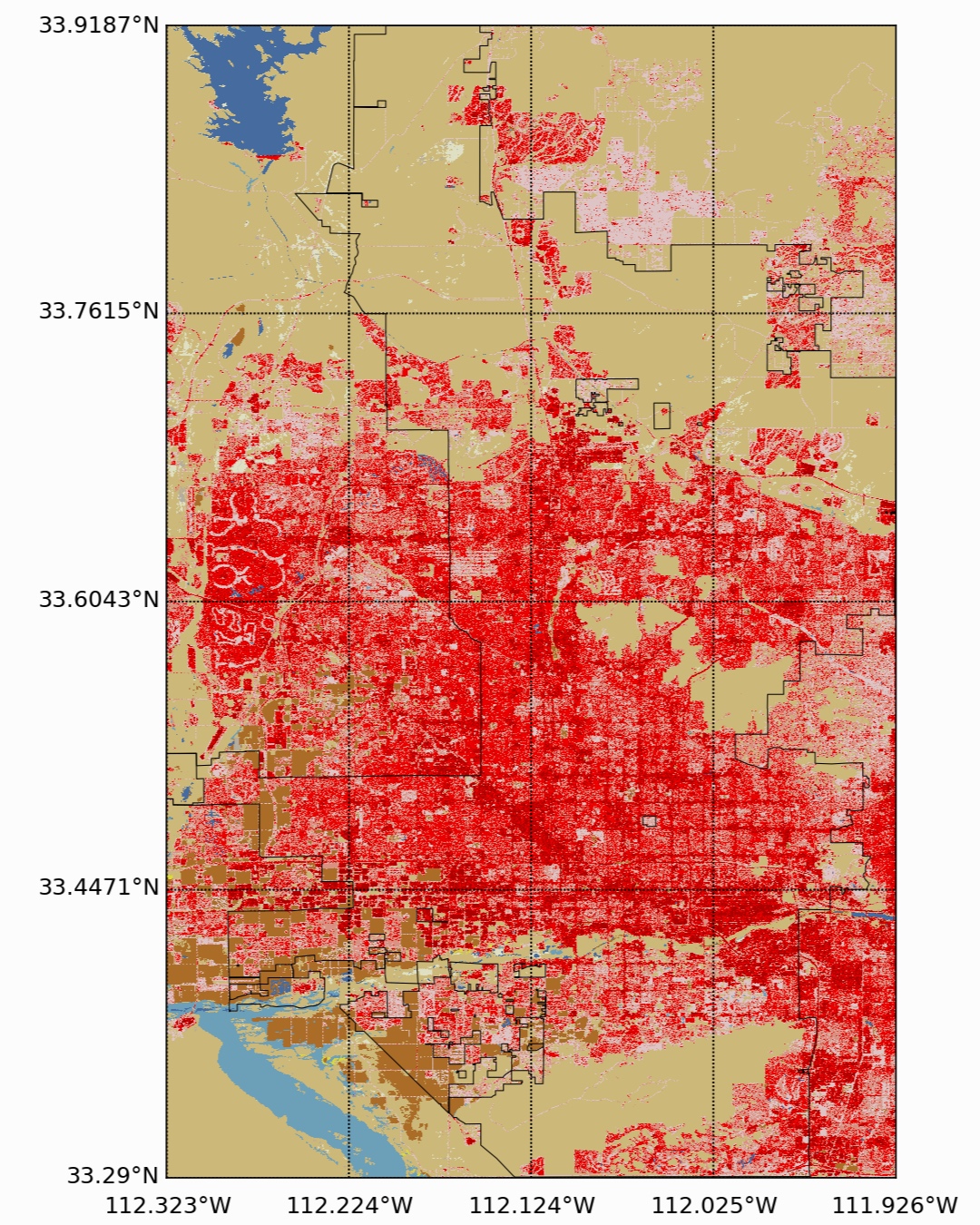
NLCD for Phoenix, AZ
In the next section, we will dive into quantifying urbanization as well as other land covers to ultimately characterize temperature profiles that are inherent to particular cities and urban areas.
If we investigate the proportion of each land cover class for New York City (excluding 0 values and water), we can get an idea of the urbanization of land for the region. The following code snippet will print out the proportion of each land cover class:
# NLCD Proportion Calculation
unique, counts = np.unique(nlcd, return_counts=True) # NLCD unique points and counts
unique,counts = unique[2:],counts[2:] # skip 0 (NaN) and 11 (water)
prop_list = []
for ii,jj in enumerate(unique):
    unq_indx = int(np.where(jj==legend)[0]) # find index
    prop_list.append(counts[ii]/np.sum(counts)) # create vector of proportions
    # print out proportion of NLCD
    print(str(leg_str[unq_indx])+': '.format(counts[ii]/np.sum(counts)))
The subsequent printout should be similar to the following:
-Developed, Open Space: 0.16
- Developed, Low Intensity: 0.19
- Developed, Medium Intensity: 0.29
- Developed High Intensity: 0.24
- Barren Land (Rock/Sand/Clay): 0.01
- Deciduous Forest: 0.04
- Evergreen Forest: 0.00
- Mixed Forest: 0.01
- Shrub/Scrub: 0.00
- Grassland/Herbaceous: 0.01
- Pasture/Hay: 0.00
- Cultivated Crops: 0.00
- Woody Wetlands: 0.02
- Emergent Herbaceous Wetlands: 0.02
These proportions add up to 1.0, which means that we have a proportion of land cover (minus water and NaN values) for the urban region. We can interpret this by using the Developed High Intensity land cover as an example. The high intensity proportion is 0.24, meaning that 24% of the land cover is highly urban for the region (NYC and some of New Jersey). Additionally, if we sum up all of the urban classes (Developed) we can state that the region is 88% urban - a striking statistic. The city of phoenix, by comparison, is only 45% urban. As we would expect, Phoenix is 47% shrub/scrub land - which is indicative of the desert-like land that surrounds it.
We can take this analysis even further by using the GOES-16 satellite pixel boundaries as clipping points to create a relationship between land cover proportion and land surface temperature (other variables as well, if desired). The method to follow is not necessarily a defined or exact process, but it can help us understand the influence that land cover has on heating of the earth’s surface.
First, we can start by bounding each GOES-16 pixel by its respective neighbors. This will allow us to clip the NLCD points by each satellite pixel’s rough bounding box. A snapshot of this happening in real-time is shown below, where a few clips have been computed and the bounding points are plotted within each GOES-16 pixel (where the pixel is defined at its center point):
Above, each satellite pixel center (black dot above) is bound by four red circles and will subsequently be filled-in by the colored rectangles. The colored rectangles represent the NLCD points contained within each GOES-16 bounded pixel (red circles). These boundings will allow us to calculate statistics relating GOES-16 data to ground parameters (NLCD). This is a powerful tool for analyzing the significance of land cover with, for our specific case, land surface temperature (LST). The code to replicate the plot above is given below, and the following plots and codes will demonstrate the implementation of the bounded colored rectangles.
import matplotlib as mpl
mpl.use('TkAgg')
import matplotlib.pyplot as plt
from matplotlib.colors import ListedColormap
from mpl_toolkits.basemap import Basemap
import numpy as np
from osgeo import gdal,ogr,osr
from netCDF4 import Dataset
import os,pyproj,rasterio

# function for calculating NLCD values in plot window
def format_coord(x, y):
    indx = np.argmin(np.abs(np.subtract(x,lons))+np.abs(np.subtract(y,lats)))
    indx = np.unravel_index(indx,np.shape(lats))
    z = nlcd[indx]
    z_str = leg_str[int(np.where(z==legend)[0])]
    return f', , NLCD:  ()'

# lat/lon reprojection from GOES-16 satellite
def lat_lon_reproj(nc_folder):
    os.chdir(nc_folder)
    full_direc = os.listdir()
    nc_files = [ii for ii in full_direc if ii.endswith('.nc')]
    g16_data_file = nc_files[0] # select .nc file
    print(nc_files[0]) # print file name

    # designate dataset
    g16nc = Dataset(g16_data_file, 'r')
    var_names = [ii for ii in g16nc.variables]
    var_name = var_names[0]

    # GOES-R projection info and retrieving relevant constants
    proj_info = g16nc.variables['goes_imager_projection']
    lon_origin = proj_info.longitude_of_projection_origin
    H = proj_info.perspective_point_height+proj_info.semi_major_axis
    r_eq = proj_info.semi_major_axis
    r_pol = proj_info.semi_minor_axis

    # grid info
    lat_rad_1d = g16nc.variables['x'][:]
    lon_rad_1d = g16nc.variables['y'][:]

    # close file when finished
    g16nc.close()
    g16nc = None

    # create meshgrid filled with radian angles
    lat_rad,lon_rad = np.meshgrid(lat_rad_1d,lon_rad_1d)

    # lat/lon calc routine from satellite radian angle vectors

    lambda_0 = (lon_origin*np.pi)/180.0

    a_var = np.power(np.sin(lat_rad),2.0) + (np.power(np.cos(lat_rad),2.0)*\
                                             (np.power(np.cos(lon_rad),2.0)+\
                                              (((r_eq*r_eq)/(r_pol*r_pol))*\
                                               np.power(np.sin(lon_rad),2.0))))
    b_var = -2.0*H*np.cos(lat_rad)*np.cos(lon_rad)
    c_var = (H**2.0)-(r_eq**2.0)

    r_s = (-1.0*b_var - np.sqrt((b_var**2)-(4.0*a_var*c_var)))/(2.0*a_var)

    s_x = r_s*np.cos(lat_rad)*np.cos(lon_rad)
    s_y = - r_s*np.sin(lat_rad)
    s_z = r_s*np.cos(lat_rad)*np.sin(lon_rad)

    # latitude and longitude projection for plotting data on traditional lat/lon maps
    lat = (180.0/np.pi)*(np.arctan(((r_eq*r_eq)/(r_pol*r_pol))*\
                                   ((s_z/np.sqrt(((H-s_x)*(H-s_x))+(s_y*s_y))))))
    lon = (lambda_0 - np.arctan(s_y/(H-s_x)))*(180.0/np.pi)

    os.chdir('../')

    return lon,lat

# grabbing data from GOES-16 satellite
def data_grab(nc_folder,nc_indx):
    os.chdir(nc_folder)
    full_direc = os.listdir()
    nc_files = [ii for ii in full_direc if ii.endswith('.nc')]
    g16_data_file = nc_files[nc_indx] # select .nc file
    print(nc_files[nc_indx]) # print file name

    # designate dataset
    g16nc = Dataset(g16_data_file, 'r')
    var_names = [ii for ii in g16nc.variables]
    var_name = var_names[0]

    # data info
    data = g16nc.variables[var_name][:]
    data_units = g16nc.variables[var_name].units
    data_time_grab = ((g16nc.time_coverage_end).replace('T',' ')).replace('Z','')
    data_long_name = g16nc.variables[var_name].long_name

    # close file when finished
    g16nc.close()
    g16nc = None

    os.chdir('../')
    # print test coordinates
    print('{} N, {} W'.format(lat[318,1849],abs(lon[318,1849])))

    return data,data_units,data_time_grab,data_long_name,var_name

##############################################
## NLCD CLIPPING
##############################################

# legend indices and strings that represent each land cover type
legend = np.array([0,11,12,21,22,23,24,31,41,42,43,51,52,71,72,73,74,81,82,90,95])
leg_str = np.array(['NaN','Open Water','Perennial Ice/Snow','Developed, Open Space','Developed, Low Intensity',
           'Developed, Medium Intensity','Developed High Intensity','Barren Land (Rock/Sand/Clay)',
           'Deciduous Forest','Evergreen Forest','Mixed Forest','Dwarf Scrub','Shrub/Scrub',
           'Grassland/Herbaceous','Sedge/Herbaceous','Lichens','Moss','Pasture/Hay','Cultivated Crops',
           'Woody Wetlands','Emergent Herbaceous Wetlands'])

# reading shapefile to set boundaries
shapefile_folder = './Borough Boundaries/'
shapefile_name = 'geo_export_ade24428-c163-42c7-9e6d-7e9743323143'
drv    = ogr.GetDriverByName('ESRI Shapefile') # define shapefile driver
ds_in  = drv.Open(shapefile_folder+shapefile_name+'.shp',0) #open shapefile
lyr_in = ds_in.GetLayer() # grab layer
sourceprj = (lyr_in.GetSpatialRef()) # input projection
targetprj = osr.SpatialReference()
targetprj.ImportFromEPSG(4326) # wanted projection
transform = osr.CoordinateTransformation(sourceprj, targetprj)
shp = lyr_in.GetExtent()
ll_x,ll_y,_ = transform.TransformPoint(shp[0],shp[2]) # reprojected bounds for city
ur_x,ur_y,_ = transform.TransformPoint(shp[1],shp[3]) # reprojected bounds for city
bbox = [ll_x,ll_y,ur_x,ur_y] # bounding box

# reproject shapefile (if correct projection, the same is return; if incorrect
# it will reproject to WGS84)
outputShapefile = shapefile_folder+shapefile_name+'_correct_CRS.shp'
if os.path.exists(outputShapefile):
    drv.DeleteDataSource(outputShapefile)
outDataSet = drv.CreateDataSource(outputShapefile)
outLayer = outDataSet.CreateLayer("correct_CRS", geom_type=ogr.wkbMultiPolygon)

# add fields
inLayerDefn = lyr_in.GetLayerDefn()
for i in range(0, inLayerDefn.GetFieldCount()):
    fieldDefn = inLayerDefn.GetFieldDefn(i)
    outLayer.CreateField(fieldDefn)

# get the output layer's feature definition
outLayerDefn = outLayer.GetLayerDefn()

inFeature = lyr_in.GetNextFeature()
while inFeature:
    # get the input geometry
    geom = inFeature.GetGeometryRef()
    # reproject the geometry
    geom.Transform(transform)
    # create a new feature
    outFeature = ogr.Feature(outLayerDefn)
    # set the geometry and attribute
    outFeature.SetGeometry(geom)
    for i in range(0, outLayerDefn.GetFieldCount()):
        outFeature.SetField(outLayerDefn.GetFieldDefn(i).GetNameRef(), inFeature.GetField(i))
    # add the feature to the shapefile
    outLayer.CreateFeature(outFeature)
    # dereference the features and get the next input feature
    outFeature = None
    inFeature = lyr_in.GetNextFeature()
    # Save and close the shapefiles
inDataSet = None
outDataSet = None

# NLCD folder
home_dir = os.getcwd() # change to NLCD folder
nlcd_filename = 'NLCD_2016_Land_Cover_L48_20190424.img' # NLCD raster
os.chdir('./NLCD_2016_Land_Cover_L48_20190424/') # location of NLCD raster

# routine for computing affine transformation for projection of lat/lon eastings
with rasterio.open(nlcd_filename) as r:
    T0 = r.transform

inproj = pyproj.Proj(init='epsg:4326') # NYC bbox projection
outproj = pyproj.Proj('+proj=aea +lat_1=29.5 +lat_2=45.5 +lat_0=23.0 '+\
                      '+lon_0=-96 +x_0=0 +y_0=0 +datum=NAD83 +towgs84=0,0,0,0 +units=m +no_defs') # NLCD proj.

# inversing bounding box coordinates to NLCD local coordinate system indices
x_ll,y_ll = ~T0*((pyproj.transform(inproj,outproj,bbox[0],bbox[1])))
x_ul,y_ul = ~T0*((pyproj.transform(inproj,outproj,bbox[0],bbox[3])))
x_lr,y_lr = ~T0*((pyproj.transform(inproj,outproj,bbox[2],bbox[1])))
x_ur,y_ur = ~T0*((pyproj.transform(inproj,outproj,bbox[2],bbox[3])))
x_span = [x_ll,x_ul,x_lr,x_ur]
y_span = [y_ll,y_ul,y_lr,y_ur]

# calculating NLCD image bounds that relate to NYC bbox
cols, rows = np.meshgrid(np.arange(r.width)[int(np.min(x_span)):int(np.max(x_span))],
                       np.arange(r.height)[int(np.min(y_span)):int(np.max(y_span))])
eastings,northings = (cols,rows)*T0

# transformation from raw projection to WGS84 lat/lon values
inproj = pyproj.Proj('+proj=aea +lat_1=29.5 +lat_2=45.5 +lat_0=23.0 +lon_0=-96 +x_0=0 +y_0=0'+\
                     ' +datum=NAD83 +towgs84=0,0,0,0 +units=m +no_defs')
outproj = pyproj.Proj(init='epsg:4326')
xvals,yvals = (eastings,northings)
lons,lats = (pyproj.transform(inproj,outproj,xvals,yvals)) # actual lats/lons

# reading NLCD data from bounds
ds = gdal.Open(nlcd_filename)
nlcd_reader = ds.GetRasterBand(1)
nlcd = nlcd_reader.ReadAsArray(int(np.min(x_span)),int(np.min(y_span)),
                               int(np.max(x_span))-int(np.min(x_span)),int(np.max(y_span))-int(np.min(y_span)))

# colormap determination and setting bounds
with rasterio.open(nlcd_filename) as r:
    cmap_in = r.colormap(1)
    cmap1 = [[np.int(jj) for jj in cmap_in[ii]] for ii in cmap_in]
    cmap_in = [[np.float(jj)/255.0 for jj in cmap_in[ii]] for ii in cmap_in]
    indx_list = np.unique(nlcd)
    r_cmap = []
    for ii in indx_list:
        r_cmap.append(cmap_in[ii])
    raster_cmap = ListedColormap(r_cmap) # defining the NLCD specific color map
    norm = mpl.colors.BoundaryNorm(indx_list, raster_cmap.N) # specifying colors based on num. unique points

##############################################
## NLCD STATISTICS SECTION
##############################################

unique, counts = np.unique(nlcd, return_counts=True) # NLCD unique points and counts
unique,counts = unique[2:],counts[2:] # skip 0 (NaN) and 11 (water)
prop_list = []
for ii,jj in enumerate(unique):
    unq_indx = int(np.where(jj==legend)[0]) # find index
    prop_list.append(counts[ii]/np.sum(counts)) # create vector of proportions
    # print out proportion of NLCD
    print(str(leg_str[unq_indx])+': '.format(counts[ii]/np.sum(counts)))

# finding boroughs from NYC shapefile
boro_array = []
for ii in range(0,(lyr_in.GetFeatureCount())):
    boro_array.append((lyr_in.GetFeature(ii)).GetField(0))

boro_unique = np.unique(boro_array)
boro_str = ['']*len(boro_unique)

##################
# routine that checks which points are inside each GOES-16 pixel
##################
os.chdir(home_dir)

# loop through boroughs to find where the points lie
fig,ax = plt.subplots(figsize=(14,8))
m = Basemap(llcrnrlon=bbox[0],llcrnrlat=bbox[1],urcrnrlon=bbox[2],
            urcrnrlat=bbox[3],resolution='i', projection='cyl')
m.readshapefile(shapefile_folder+shapefile_name+'_correct_CRS',
                'nyc_shapefile')
m.drawmapboundary(fill_color='#bdd5d5')
parallels = np.linspace(bbox[1],bbox[3],5.) # latitudes
m.drawparallels(parallels,labels=[True,False,False,False],fontsize=12)
meridians = np.linspace(bbox[0],bbox[2],5.) # longitudes
m.drawmeridians(meridians,labels=[False,False,False,True],fontsize=12)

# GOES-16 folder and lat/lon reprojection + data reader
nc_folder = './GOES_files/' # define folder where .nc files are located
lon,lat = lat_lon_reproj(nc_folder)

file_indx = 18 # be sure to pick the correct file. Make sure the file is not too big either,
# some of the bands create large files (stick to band 7-16)

data,data_units,data_time_grab,data_long_name,var_name = data_grab(nc_folder,file_indx)

##################
# clipping lat/lon/data vectors to shapefile bounds
##################

llcrnr_loc_x = np.ma.argmin(np.ma.min(np.abs(np.ma.subtract(lon,bbox[0]))+\
                                      np.abs(np.ma.subtract(lat,bbox[1])),0))
llcrnr_loc = (np.ma.argmin(np.abs(np.ma.subtract(lon,bbox[0]))+\
                           np.abs(np.ma.subtract(lat,bbox[1])),0))[llcrnr_loc_x]

ulcrnr_loc_x = np.ma.argmin(np.ma.min(np.abs(np.ma.subtract(lon,bbox[0]))+\
                                      np.abs(np.ma.subtract(lat,bbox[3])),0))
ulcrnr_loc = (np.ma.argmin(np.abs(np.ma.subtract(lon,bbox[0]))+\
                           np.abs(np.ma.subtract(lat,bbox[3])),0))[ulcrnr_loc_x]

lrcrnr_loc_x = np.ma.argmin(np.ma.min(np.abs(np.ma.subtract(lon,bbox[2]))+\
                                      np.abs(np.ma.subtract(lat,bbox[1])),0))
lrcrnr_loc = (np.ma.argmin(np.abs(np.ma.subtract(lon,bbox[2]))+\
                           np.abs(np.ma.subtract(lat,bbox[1])),0))[lrcrnr_loc_x]

urcrnr_loc_x = np.ma.argmin(np.ma.min(np.abs(np.ma.subtract(lon,bbox[2]))+\
                                      np.abs(np.ma.subtract(lat,bbox[3])),0))
urcrnr_loc = (np.ma.argmin(np.abs(np.ma.subtract(lon,bbox[2]))+\
                           np.abs(np.ma.subtract(lat,bbox[3])),0))[urcrnr_loc_x]

x_bounds = [llcrnr_loc_x,ulcrnr_loc_x,lrcrnr_loc_x,urcrnr_loc_x]
y_bounds = [llcrnr_loc,ulcrnr_loc,lrcrnr_loc,urcrnr_loc]

plot_bounds = [np.min(x_bounds),np.min(y_bounds),np.max(x_bounds)+1,np.max(y_bounds)+1]

lat_clip = lat[plot_bounds[1]:plot_bounds[3],plot_bounds[0]:plot_bounds[2]]
lon_clip = lon[plot_bounds[1]:plot_bounds[3],plot_bounds[0]:plot_bounds[2]]
dat_clip = data[plot_bounds[1]:plot_bounds[3],plot_bounds[0]:plot_bounds[2]]

[m.plot(jj,ii,marker='o',linestyle='',color='k') for ii,jj in zip(lat_clip,lon_clip)]
# looping through points to find NLCD stats for each pixel

for mm in range(1,(np.shape(dat_clip)[0])-1):
    for nn in range(1,(np.shape(dat_clip)[1])-1):
        feat_bbox = [-np.abs((-lon_clip[mm,nn-1]+lon_clip[mm,nn])/2.0)+lon_clip[mm,nn],
                     np.abs((-lon_clip[mm,nn+1]+lon_clip[mm,nn])/2.0)+lon_clip[mm,nn],
                     -np.abs((-lat_clip[mm-1,nn]+lat_clip[mm,nn])/2.0)+lat_clip[mm,nn],
                     np.abs((-lat_clip[mm+1,nn]+lat_clip[mm,nn])/2.0)+lat_clip[mm,nn]]
        m.plot(feat_bbox[0],feat_bbox[2],marker='o',linestyle='',color='r')
        m.plot(feat_bbox[1],feat_bbox[2],marker='o',linestyle='',color='r')
        m.plot(feat_bbox[0],feat_bbox[3],marker='o',linestyle='',color='r')
        m.plot(feat_bbox[1],feat_bbox[3],marker='o',linestyle='',color='r')

        crop_lats = lats[(lons>feat_bbox[0]) & (lons<feat_bbox[1]) & (lats>feat_bbox[2]) & (lats<feat_bbox[3])]
        crop_lons = lons[(lons>feat_bbox[0]) & (lons<feat_bbox[1]) & (lats>feat_bbox[2]) & (lats<feat_bbox[3])]
        crop_nlcd = nlcd[(lons>feat_bbox[0]) & (lons<feat_bbox[1]) & (lats>feat_bbox[2]) & (lats<feat_bbox[3])]

        m.plot(crop_lons,crop_lats,marker='.',linestyle='',markersize=2.5)
        if mm==3 and nn==12:
            plt.savefig('nlcd_mapper_goes16_pixel_example_scatter.png',dpi=150,facecolor=[252/255,252/255,252/255])
            break
        plt.pause(0.05)
If we wanted to map out how urban each satellite pixel was, we can use the bounding method shown above along with the standard satellite mapping technique, and end up with the following pixel mapping of urbanization:
In the image above, I’ve done a few things:
Technically, the figure is plotted with a shift to align the colors to the respective black dot satellite pixel centers. This is the true visualization of the satellite information. This is necessary because of the Python function ‘pcolormesh()’ which uses the top right corner as the input.
The urbanization percentage above uses only the Developed parameters of the NLCD
The urbanization is a linear combination of the developed parameters bound by each GOES-16 satellite pixel’s rough bounding
This method of combining the NLCD using the GOES-16 satellite pixel information will be the basis for the analysis that follow, which entails relating land cover proportion to LST data. This will give us an idea of how each land cover class affects surface temperature, indicating whether land cover is directly correlated to surface temperature or not.
The code for the urbanization of satellite pixels is given below:
import matplotlib as mpl
mpl.use('TkAgg')
import matplotlib.pyplot as plt
from matplotlib.colors import ListedColormap
from mpl_toolkits.basemap import Basemap
import numpy as np
from osgeo import gdal,ogr,osr
from netCDF4 import Dataset
import os,pyproj,rasterio

# function for calculating NLCD values in plot window
def format_coord(x, y):
    indx = np.argmin(np.abs(np.subtract(x,lons))+np.abs(np.subtract(y,lats)))
    indx = np.unravel_index(indx,np.shape(lats))
    z = nlcd[indx]
    z_str = leg_str[int(np.where(z==legend)[0])]
    return f', , NLCD:  ()'

# lat/lon reprojection from GOES-16 satellite
def lat_lon_reproj(nc_folder):
    os.chdir(nc_folder)
    full_direc = os.listdir()
    nc_files = [ii for ii in full_direc if ii.endswith('.nc')]
    g16_data_file = nc_files[0] # select .nc file
    print(nc_files[0]) # print file name

    # designate dataset
    g16nc = Dataset(g16_data_file, 'r')
    var_names = [ii for ii in g16nc.variables]
    var_name = var_names[0]

    # GOES-R projection info and retrieving relevant constants
    proj_info = g16nc.variables['goes_imager_projection']
    lon_origin = proj_info.longitude_of_projection_origin
    H = proj_info.perspective_point_height+proj_info.semi_major_axis
    r_eq = proj_info.semi_major_axis
    r_pol = proj_info.semi_minor_axis

    # grid info
    lat_rad_1d = g16nc.variables['x'][:]
    lon_rad_1d = g16nc.variables['y'][:]

    # close file when finished
    g16nc.close()
    g16nc = None

    # create meshgrid filled with radian angles
    lat_rad,lon_rad = np.meshgrid(lat_rad_1d,lon_rad_1d)

    # lat/lon calc routine from satellite radian angle vectors

    lambda_0 = (lon_origin*np.pi)/180.0

    a_var = np.power(np.sin(lat_rad),2.0) + (np.power(np.cos(lat_rad),2.0)*\
                                             (np.power(np.cos(lon_rad),2.0)+\
                                              (((r_eq*r_eq)/(r_pol*r_pol))*\
                                               np.power(np.sin(lon_rad),2.0))))
    b_var = -2.0*H*np.cos(lat_rad)*np.cos(lon_rad)
    c_var = (H**2.0)-(r_eq**2.0)

    r_s = (-1.0*b_var - np.sqrt((b_var**2)-(4.0*a_var*c_var)))/(2.0*a_var)

    s_x = r_s*np.cos(lat_rad)*np.cos(lon_rad)
    s_y = - r_s*np.sin(lat_rad)
    s_z = r_s*np.cos(lat_rad)*np.sin(lon_rad)

    # latitude and longitude projection for plotting data on traditional lat/lon maps
    lat = (180.0/np.pi)*(np.arctan(((r_eq*r_eq)/(r_pol*r_pol))*\
                                   ((s_z/np.sqrt(((H-s_x)*(H-s_x))+(s_y*s_y))))))
    lon = (lambda_0 - np.arctan(s_y/(H-s_x)))*(180.0/np.pi)

    os.chdir('../')

    return lon,lat

# grabbing data from GOES-16 satellite
def data_grab(nc_folder,nc_indx):
    os.chdir(nc_folder)
    full_direc = os.listdir()
    nc_files = [ii for ii in full_direc if ii.endswith('.nc')]
    g16_data_file = nc_files[nc_indx] # select .nc file
    print(nc_files[nc_indx]) # print file name

    # designate dataset
    g16nc = Dataset(g16_data_file, 'r')
    var_names = [ii for ii in g16nc.variables]
    var_name = var_names[0]

    # data info
    data = g16nc.variables[var_name][:]
    data_units = g16nc.variables[var_name].units
    data_time_grab = ((g16nc.time_coverage_end).replace('T',' ')).replace('Z','')
    data_long_name = g16nc.variables[var_name].long_name

    # close file when finished
    g16nc.close()
    g16nc = None

    os.chdir('../')
    # print test coordinates
    print('{} N, {} W'.format(lat[318,1849],abs(lon[318,1849])))

    return data,data_units,data_time_grab,data_long_name,var_name

##############################################
## NLCD CLIPPING
##############################################

# legend indices and strings that represent each land cover type
legend = np.array([0,11,12,21,22,23,24,31,41,42,43,51,52,71,72,73,74,81,82,90,95])
leg_str = np.array(['NaN','Open Water','Perennial Ice/Snow','Developed, Open Space','Developed, Low Intensity',
           'Developed, Medium Intensity','Developed High Intensity','Barren Land (Rock/Sand/Clay)',
           'Deciduous Forest','Evergreen Forest','Mixed Forest','Dwarf Scrub','Shrub/Scrub',
           'Grassland/Herbaceous','Sedge/Herbaceous','Lichens','Moss','Pasture/Hay','Cultivated Crops',
           'Woody Wetlands','Emergent Herbaceous Wetlands'])

# reading shapefile to set boundaries
shapefile_folder = './Borough Boundaries/'
shapefile_name = 'geo_export_ade24428-c163-42c7-9e6d-7e9743323143'
drv    = ogr.GetDriverByName('ESRI Shapefile') # define shapefile driver
ds_in  = drv.Open(shapefile_folder+shapefile_name+'.shp',0) #open shapefile
lyr_in = ds_in.GetLayer() # grab layer
sourceprj = (lyr_in.GetSpatialRef()) # input projection
targetprj = osr.SpatialReference()
targetprj.ImportFromEPSG(4326) # wanted projection
transform = osr.CoordinateTransformation(sourceprj, targetprj)
shp = lyr_in.GetExtent()
ll_x,ll_y,_ = transform.TransformPoint(shp[0],shp[2]) # reprojected bounds for city
ur_x,ur_y,_ = transform.TransformPoint(shp[1],shp[3]) # reprojected bounds for city
bbox = [ll_x,ll_y,ur_x,ur_y] # bounding box

# reproject shapefile (if correct projection, the same is return; if incorrect
# it will reproject to WGS84)
outputShapefile = shapefile_folder+shapefile_name+'_correct_CRS.shp'
if os.path.exists(outputShapefile):
    drv.DeleteDataSource(outputShapefile)
outDataSet = drv.CreateDataSource(outputShapefile)
outLayer = outDataSet.CreateLayer("correct_CRS", geom_type=ogr.wkbMultiPolygon)

# add fields
inLayerDefn = lyr_in.GetLayerDefn()
for i in range(0, inLayerDefn.GetFieldCount()):
    fieldDefn = inLayerDefn.GetFieldDefn(i)
    outLayer.CreateField(fieldDefn)

# get the output layer's feature definition
outLayerDefn = outLayer.GetLayerDefn()

inFeature = lyr_in.GetNextFeature()
while inFeature:
    # get the input geometry
    geom = inFeature.GetGeometryRef()
    # reproject the geometry
    geom.Transform(transform)
    # create a new feature
    outFeature = ogr.Feature(outLayerDefn)
    # set the geometry and attribute
    outFeature.SetGeometry(geom)
    for i in range(0, outLayerDefn.GetFieldCount()):
        outFeature.SetField(outLayerDefn.GetFieldDefn(i).GetNameRef(), inFeature.GetField(i))
    # add the feature to the shapefile
    outLayer.CreateFeature(outFeature)
    # dereference the features and get the next input feature
    outFeature = None
    inFeature = lyr_in.GetNextFeature()
    # Save and close the shapefiles
inDataSet = None
outDataSet = None

# NLCD folder
home_dir = os.getcwd() # change to NLCD folder
nlcd_filename = 'NLCD_2016_Land_Cover_L48_20190424.img' # NLCD raster
os.chdir('./NLCD_2016_Land_Cover_L48_20190424/') # location of NLCD raster

# routine for computing affine transformation for projection of lat/lon eastings
with rasterio.open(nlcd_filename) as r:
    T0 = r.transform

inproj = pyproj.Proj(init='epsg:4326') # NYC bbox projection
outproj = pyproj.Proj('+proj=aea +lat_1=29.5 +lat_2=45.5 +lat_0=23.0 '+\
                      '+lon_0=-96 +x_0=0 +y_0=0 +datum=NAD83 +towgs84=0,0,0,0 +units=m +no_defs') # NLCD proj.

# inversing bounding box coordinates to NLCD local coordinate system indices
x_ll,y_ll = ~T0*((pyproj.transform(inproj,outproj,bbox[0],bbox[1])))
x_ul,y_ul = ~T0*((pyproj.transform(inproj,outproj,bbox[0],bbox[3])))
x_lr,y_lr = ~T0*((pyproj.transform(inproj,outproj,bbox[2],bbox[1])))
x_ur,y_ur = ~T0*((pyproj.transform(inproj,outproj,bbox[2],bbox[3])))
x_span = [x_ll,x_ul,x_lr,x_ur]
y_span = [y_ll,y_ul,y_lr,y_ur]

# calculating NLCD image bounds that relate to NYC bbox
cols, rows = np.meshgrid(np.arange(r.width)[int(np.min(x_span)):int(np.max(x_span))],
                       np.arange(r.height)[int(np.min(y_span)):int(np.max(y_span))])
eastings,northings = (cols,rows)*T0

# transformation from raw projection to WGS84 lat/lon values
inproj = pyproj.Proj('+proj=aea +lat_1=29.5 +lat_2=45.5 +lat_0=23.0 +lon_0=-96 +x_0=0 +y_0=0'+\
                     ' +datum=NAD83 +towgs84=0,0,0,0 +units=m +no_defs')
outproj = pyproj.Proj(init='epsg:4326')
xvals,yvals = (eastings,northings)
lons,lats = (pyproj.transform(inproj,outproj,xvals,yvals)) # actual lats/lons

# reading NLCD data from bounds
ds = gdal.Open(nlcd_filename)
nlcd_reader = ds.GetRasterBand(1)
nlcd = nlcd_reader.ReadAsArray(int(np.min(x_span)),int(np.min(y_span)),
                               int(np.max(x_span))-int(np.min(x_span)),int(np.max(y_span))-int(np.min(y_span)))

# colormap determination and setting bounds
with rasterio.open(nlcd_filename) as r:
    cmap_in = r.colormap(1)
    cmap1 = [[np.int(jj) for jj in cmap_in[ii]] for ii in cmap_in]
    cmap_in = [[np.float(jj)/255.0 for jj in cmap_in[ii]] for ii in cmap_in]
    indx_list = np.unique(nlcd)
    r_cmap = []
    for ii in indx_list:
        r_cmap.append(cmap_in[ii])
    raster_cmap = ListedColormap(r_cmap) # defining the NLCD specific color map
    norm = mpl.colors.BoundaryNorm(indx_list, raster_cmap.N) # specifying colors based on num. unique points

##############################################
## NLCD STATISTICS SECTION
##############################################

unique, counts = np.unique(nlcd, return_counts=True) # NLCD unique points and counts
unique,counts = unique[2:],counts[2:] # skip 0 (NaN) and 11 (water)
prop_list = []
for ii,jj in enumerate(unique):
    unq_indx = int(np.where(jj==legend)[0]) # find index
    prop_list.append(counts[ii]/np.sum(counts)) # create vector of proportions
    # print out proportion of NLCD
    print(str(leg_str[unq_indx])+': '.format(counts[ii]/np.sum(counts)))

# finding boroughs from NYC shapefile
boro_array = []
for ii in range(0,(lyr_in.GetFeatureCount())):
    boro_array.append((lyr_in.GetFeature(ii)).GetField(0))

boro_unique = np.unique(boro_array)
boro_str = ['']*len(boro_unique)

##################
# routine that checks which points are inside each GOES-16 pixel
##################
os.chdir(home_dir)

# loop through boroughs to find where the points lie
fig,ax = plt.subplots(figsize=(14,8))
m = Basemap(llcrnrlon=bbox[0],llcrnrlat=bbox[1],urcrnrlon=bbox[2],
            urcrnrlat=bbox[3],resolution='i', projection='cyl')
m.readshapefile(shapefile_folder+shapefile_name+'_correct_CRS',
                'nyc_shapefile')
m.drawmapboundary(fill_color='#bdd5d5')
parallels = np.linspace(bbox[1],bbox[3],5.) # latitudes
m.drawparallels(parallels,labels=[True,False,False,False],fontsize=12)
meridians = np.linspace(bbox[0],bbox[2],5.) # longitudes
m.drawmeridians(meridians,labels=[False,False,False,True],fontsize=12)

# GOES-16 folder and lat/lon reprojection + data reader
nc_folder = './GOES_files/' # define folder where .nc files are located
lon,lat = lat_lon_reproj(nc_folder)

file_indx = 18 # be sure to pick the correct file. Make sure the file is not too big either,
# some of the bands create large files (stick to band 7-16)

data,data_units,data_time_grab,data_long_name,var_name = data_grab(nc_folder,file_indx)

##################
# clipping satellite lat/lon/data vectors to shapefile bounds
##################

llcrnr_loc_x = np.ma.argmin(np.ma.min(np.abs(np.ma.subtract(lon,bbox[0]))+\
                                      np.abs(np.ma.subtract(lat,bbox[1])),0))
llcrnr_loc = (np.ma.argmin(np.abs(np.ma.subtract(lon,bbox[0]))+\
                           np.abs(np.ma.subtract(lat,bbox[1])),0))[llcrnr_loc_x]

ulcrnr_loc_x = np.ma.argmin(np.ma.min(np.abs(np.ma.subtract(lon,bbox[0]))+\
                                      np.abs(np.ma.subtract(lat,bbox[3])),0))
ulcrnr_loc = (np.ma.argmin(np.abs(np.ma.subtract(lon,bbox[0]))+\
                           np.abs(np.ma.subtract(lat,bbox[3])),0))[ulcrnr_loc_x]

lrcrnr_loc_x = np.ma.argmin(np.ma.min(np.abs(np.ma.subtract(lon,bbox[2]))+\
                                      np.abs(np.ma.subtract(lat,bbox[1])),0))
lrcrnr_loc = (np.ma.argmin(np.abs(np.ma.subtract(lon,bbox[2]))+\
                           np.abs(np.ma.subtract(lat,bbox[1])),0))[lrcrnr_loc_x]

urcrnr_loc_x = np.ma.argmin(np.ma.min(np.abs(np.ma.subtract(lon,bbox[2]))+\
                                      np.abs(np.ma.subtract(lat,bbox[3])),0))
urcrnr_loc = (np.ma.argmin(np.abs(np.ma.subtract(lon,bbox[2]))+\
                           np.abs(np.ma.subtract(lat,bbox[3])),0))[urcrnr_loc_x]

x_bounds = [llcrnr_loc_x,ulcrnr_loc_x,lrcrnr_loc_x,urcrnr_loc_x]
y_bounds = [llcrnr_loc,ulcrnr_loc,lrcrnr_loc,urcrnr_loc]

plot_bounds = [np.min(x_bounds),np.min(y_bounds),np.max(x_bounds)+1,np.max(y_bounds)+1]

lat_clip = lat[plot_bounds[1]:plot_bounds[3],plot_bounds[0]:plot_bounds[2]]
lon_clip = lon[plot_bounds[1]:plot_bounds[3],plot_bounds[0]:plot_bounds[2]]
dat_clip = data[plot_bounds[1]:plot_bounds[3],plot_bounds[0]:plot_bounds[2]]

[m.plot(jj,ii,marker='o',linestyle='',color='k') for ii,jj in zip(lat_clip,lon_clip)]
# looping through points to find NLCD stats for each pixel

goes_nlcd_pix = np.zeros(((np.shape(dat_clip)[0]),(np.shape(dat_clip)[1])))
lats_shift,lons_shift = np.array(lat_clip),np.array(lon_clip)
for mm in range(1,(np.shape(dat_clip)[0])-1):
    for nn in range(1,(np.shape(dat_clip)[1])-1):
        feat_bbox = [-np.abs((-lon_clip[mm,nn-1]+lon_clip[mm,nn])/2.0)+lon_clip[mm,nn],
                     np.abs((-lon_clip[mm,nn+1]+lon_clip[mm,nn])/2.0)+lon_clip[mm,nn],
                     -np.abs((-lat_clip[mm-1,nn]+lat_clip[mm,nn])/2.0)+lat_clip[mm,nn],
                     np.abs((-lat_clip[mm+1,nn]+lat_clip[mm,nn])/2.0)+lat_clip[mm,nn]]
        m.plot(feat_bbox[0],feat_bbox[2],marker='o',linestyle='',color='r')
        m.plot(feat_bbox[1],feat_bbox[2],marker='o',linestyle='',color='r')
        m.plot(feat_bbox[0],feat_bbox[3],marker='o',linestyle='',color='r')
        m.plot(feat_bbox[1],feat_bbox[3],marker='o',linestyle='',color='r')

        crop_lats = lats[(lons>feat_bbox[0]) & (lons<feat_bbox[1]) & (lats>feat_bbox[2]) & (lats<feat_bbox[3])]
        crop_lons = lons[(lons>feat_bbox[0]) & (lons<feat_bbox[1]) & (lats>feat_bbox[2]) & (lats<feat_bbox[3])]
        crop_nlcd = nlcd[(lons>feat_bbox[0]) & (lons<feat_bbox[1]) & (lats>feat_bbox[2]) & (lats<feat_bbox[3])]

        nlcd_unq,nlcd_counts = np.unique(crop_nlcd,return_counts=True)
        urb_count,tot_sum = 0,0
        for unq_iter,unq_val in enumerate(nlcd_unq):
            if unq_val==0 or unq_val==11:
                continue
            if unq_val==21 or unq_val==22 or unq_val==23 or unq_val==24:
                urb_count+=nlcd_counts[unq_iter]

            tot_sum+=nlcd_counts[unq_iter]
        lats_shift[mm,nn] = feat_bbox[3]
        lons_shift[mm,nn] = feat_bbox[0]
        goes_nlcd_pix[mm,nn] = np.divide(urb_count,tot_sum)*100.0

m.pcolormesh(lons_shift,lats_shift,goes_nlcd_pix,latlon=True,cmap='jet',alpha=0.8)
cb = m.colorbar()

data_units = ((data_units.replace('-','^{-')).replace('1','1}')).replace('2','2}')
plt.rc('text', usetex=True)
cb.set_label('Urbanization [%]',fontsize=18)
plt.title('Urbanization in New York City by Satellite Pixel',fontsize=14)
plt.tight_layout()
plt.savefig('nyc_urbanization_pixels.png',dpi=150,
            facecolor=[252/255,252/255,252/255]) # uncomment to save figure

plt.show()
Below is the historical weather from July 2019, which coincides with a heat wave in the north east. We will be using LST data from the heat wave period to correlate surface temperatures from different land cover classes that correspond to each NYC satellite pixel.
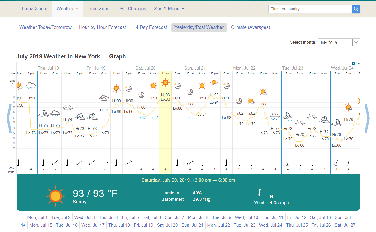
Weather History taken from https://www.timeanddate.com/weather/usa/new-york/historic?month=7&year=2019
During the heat wave, we can investigate the heating of each land cover by comparing the proportion of land cover to the deviation from the city-averaged LST. This looks like the following for highly developed areas in New York City:

The figure above tells us that as we increase the high intensity developed areas of a satellite pixel, the surface temperature increases quite a bit from the rest of the land cover types. This has huge implications for urbanization and urban planning, indicating that if we continue to build high density cities, we could be producing warmer and warmer urban regions, which can have negative effects on the population of such cities.
Conversely, if we investigate less built-up land cover, we can see a slightly different result:

The low intensity urban land cover suggests that less built-up areas result in less net heating of the surface, something that could be useful when deciding how densely to build an urban area.
Furthermore, if we investigate the city of Phoenix, AZ and its highly-developed regions, the net heating of its urbanized surface can seen as an even more severe version of New York City:

The plot above suggests that Phoenix and its high intensity developed land cover results in a net 2K increase in LST.
If we look at the non-urban cropland area surrounding the dense regions of Phoenix, we can see the cooling effects of non-urban regions:

We can see that the effects of urbanization can result in an overall heating of the land surface, specifically when the area is considered high intensity. We can also the neutral effects of lower intensity urbanization and the net cooling effects of specific natural land cover (in the case of Phoenix: cultivated crops). These findings could be important for minimizing urbanization effects on global temperatures and beneficial for the general public, specifically around extreme heat events.
The code to reproduce the plots above is given below:
import matplotlib as mpl
mpl.use('TkAgg')
import matplotlib.pyplot as plt
from matplotlib.colors import ListedColormap
from mpl_toolkits.basemap import Basemap
import numpy as np
from osgeo import gdal,ogr,osr
from netCDF4 import Dataset
import os,pyproj,rasterio

plt.style.use('ggplot')

# function for calculating NLCD values in plot window
def format_coord(x, y):
    indx = np.argmin(np.abs(np.subtract(x,lons))+np.abs(np.subtract(y,lats)))
    indx = np.unravel_index(indx,np.shape(lats))
    z = nlcd[indx]
    z_str = leg_str[int(np.where(z==legend)[0])]
    return f'{x:1.4f}, {y:1.4f}, NLCD: {z_str} ({z:1.0f})'

# lat/lon reprojection from GOES-16 satellite
def lat_lon_reproj(nc_folder):
    os.chdir(nc_folder)
    full_direc = os.listdir()
    nc_files = [ii for ii in full_direc if ii.endswith('.nc')]
    g16_data_file = nc_files[0] # select .nc file
    print(nc_files[0]) # print file name

    # designate dataset
    g16nc = Dataset(g16_data_file, 'r')
    var_names = [ii for ii in g16nc.variables]
    var_name = var_names[0]

    # GOES-R projection info and retrieving relevant constants
    proj_info = g16nc.variables['goes_imager_projection']
    lon_origin = proj_info.longitude_of_projection_origin
    H = proj_info.perspective_point_height+proj_info.semi_major_axis
    r_eq = proj_info.semi_major_axis
    r_pol = proj_info.semi_minor_axis

    # grid info
    lat_rad_1d = g16nc.variables['x'][:]
    lon_rad_1d = g16nc.variables['y'][:]

    # close file when finished
    g16nc.close()
    g16nc = None

    # create meshgrid filled with radian angles
    lat_rad,lon_rad = np.meshgrid(lat_rad_1d,lon_rad_1d)

    # lat/lon calc routine from satellite radian angle vectors

    lambda_0 = (lon_origin*np.pi)/180.0

    a_var = np.power(np.sin(lat_rad),2.0) + (np.power(np.cos(lat_rad),2.0)*\
                                             (np.power(np.cos(lon_rad),2.0)+\
                                              (((r_eq*r_eq)/(r_pol*r_pol))*\
                                               np.power(np.sin(lon_rad),2.0))))
    b_var = -2.0*H*np.cos(lat_rad)*np.cos(lon_rad)
    c_var = (H**2.0)-(r_eq**2.0)

    r_s = (-1.0*b_var - np.sqrt((b_var**2)-(4.0*a_var*c_var)))/(2.0*a_var)

    s_x = r_s*np.cos(lat_rad)*np.cos(lon_rad)
    s_y = - r_s*np.sin(lat_rad)
    s_z = r_s*np.cos(lat_rad)*np.sin(lon_rad)

    # latitude and longitude projection for plotting data on traditional lat/lon maps
    lat = (180.0/np.pi)*(np.arctan(((r_eq*r_eq)/(r_pol*r_pol))*\
                                   ((s_z/np.sqrt(((H-s_x)*(H-s_x))+(s_y*s_y))))))
    lon = (lambda_0 - np.arctan(s_y/(H-s_x)))*(180.0/np.pi)

    os.chdir('../')

    return lon,lat

# grabbing data from GOES-16 satellite
def data_grab(nc_folder,nc_indx):
    os.chdir(nc_folder)
    full_direc = os.listdir()
    nc_files = [ii for ii in full_direc if ii.endswith('.nc')]
    g16_data_file = nc_files[nc_indx] # select .nc file
    print(nc_files[nc_indx]) # print file name

    # designate dataset
    g16nc = Dataset(g16_data_file, 'r')
    var_names = [ii for ii in g16nc.variables]
    var_name = var_names[0]

    # data info
    data = g16nc.variables[var_name][:]
    data_units = g16nc.variables[var_name].units
    data_time_grab = ((g16nc.time_coverage_end).replace('T',' ')).replace('Z','')
    data_long_name = g16nc.variables[var_name].long_name

    # close file when finished
    g16nc.close()
    g16nc = None

    os.chdir('../')
    # print test coordinates
    print('{} N, {} W'.format(lat[318,1849],abs(lon[318,1849])))

    return data,data_units,data_time_grab,data_long_name,var_name

##############################################
## NLCD CLIPPING
##############################################

# legend indices and strings that represent each land cover type
legend = np.array([0,11,12,21,22,23,24,31,41,42,43,51,52,71,72,73,74,81,82,90,95])
leg_str = np.array(['NaN','Open Water','Perennial Ice/Snow','Developed, Open Space','Developed, Low Intensity',
           'Developed, Medium Intensity','Developed High Intensity','Barren Land (Rock/Sand/Clay)',
           'Deciduous Forest','Evergreen Forest','Mixed Forest','Dwarf Scrub','Shrub/Scrub',
           'Grassland/Herbaceous','Sedge/Herbaceous','Lichens','Moss','Pasture/Hay','Cultivated Crops',
           'Woody Wetlands','Emergent Herbaceous Wetlands'])

# reading shapefile to set boundaries
city_name = 'New York City'
shapefile_folder = './nyc/'
shapefile_name = (os.listdir(shapefile_folder)[0]).split('.')[0]
drv    = ogr.GetDriverByName('ESRI Shapefile') # define shapefile driver
ds_in  = drv.Open(shapefile_folder+shapefile_name+'.shp',0) #open shapefile
lyr_in = ds_in.GetLayer() # grab layer
sourceprj = (lyr_in.GetSpatialRef()) # input projection
targetprj = osr.SpatialReference()
targetprj.ImportFromEPSG(4326) # wanted projection
transform = osr.CoordinateTransformation(sourceprj, targetprj)
shp = lyr_in.GetExtent()
ll_x,ll_y,_ = transform.TransformPoint(shp[0],shp[2]) # reprojected bounds for city
ur_x,ur_y,_ = transform.TransformPoint(shp[1],shp[3]) # reprojected bounds for city
bbox = [ll_x,ll_y,ur_x,ur_y] # bounding box

# reproject shapefile (if correct projection, the same is return; if incorrect
# it will reproject to WGS84)
outputShapefile = shapefile_folder+shapefile_name+'_correct_CRS.shp'
if os.path.exists(outputShapefile):
    drv.DeleteDataSource(outputShapefile)
outDataSet = drv.CreateDataSource(outputShapefile)
outLayer = outDataSet.CreateLayer("correct_CRS", geom_type=ogr.wkbMultiPolygon)

# add fields
inLayerDefn = lyr_in.GetLayerDefn()
for i in range(0, inLayerDefn.GetFieldCount()):
    fieldDefn = inLayerDefn.GetFieldDefn(i)
    outLayer.CreateField(fieldDefn)

# get the output layer's feature definition
outLayerDefn = outLayer.GetLayerDefn()

inFeature = lyr_in.GetNextFeature()
while inFeature:
    # get the input geometry
    geom = inFeature.GetGeometryRef()
    # reproject the geometry
    geom.Transform(transform)
    # create a new feature
    outFeature = ogr.Feature(outLayerDefn)
    # set the geometry and attribute
    outFeature.SetGeometry(geom)
    for i in range(0, outLayerDefn.GetFieldCount()):
        outFeature.SetField(outLayerDefn.GetFieldDefn(i).GetNameRef(), inFeature.GetField(i))
    # add the feature to the shapefile
    outLayer.CreateFeature(outFeature)
    # dereference the features and get the next input feature
    outFeature = None
    inFeature = lyr_in.GetNextFeature()
    # Save and close the shapefiles
inDataSet = None
outDataSet = None

# shapefile plotter
fig,ax = plt.subplots(figsize=(14,8))
m = Basemap(llcrnrlon=bbox[0],llcrnrlat=bbox[1],urcrnrlon=bbox[2],
            urcrnrlat=bbox[3],resolution='i', projection='cyl')
m.readshapefile(shapefile_folder+shapefile_name+'_correct_CRS',
                'curr_shapefile')
m.drawmapboundary(fill_color='#bdd5d5')
parallels = np.linspace(bbox[1],bbox[3],5.) # latitudes
m.drawparallels(parallels,labels=[True,False,False,False],fontsize=12)
meridians = np.linspace(bbox[0],bbox[2],5.) # longitudes
m.drawmeridians(meridians,labels=[False,False,False,True],fontsize=12)
plt.show()

# GOES lat/lon grid file for CONUS
nc_folder = './GOES_files/' # define folder where .nc files are located
lon,lat = lat_lon_reproj(nc_folder)

# NLCD folder
home_dir = os.getcwd() # change to NLCD folder
nlcd_filename = 'NLCD_2016_Land_Cover_L48_20190424.img' # NLCD raster
os.chdir('../../NLCD/NLCD_2016_Land_Cover_L48_20190424/') # location of NLCD raster

# routine for computing affine transformation for projection of lat/lon eastings
with rasterio.open(nlcd_filename) as r:
    T0 = r.transform

inproj = pyproj.Proj(init='epsg:4326') # NYC bbox projection
outproj = pyproj.Proj('+proj=aea +lat_1=29.5 +lat_2=45.5 +lat_0=23.0 '+\
                      '+lon_0=-96 +x_0=0 +y_0=0 +datum=NAD83 +towgs84=0,0,0,0 +units=m +no_defs') # NLCD proj.

# inversing bounding box coordinates to NLCD local coordinate system indices
x_ll,y_ll = ~T0*((pyproj.transform(inproj,outproj,bbox[0],bbox[1])))
x_ul,y_ul = ~T0*((pyproj.transform(inproj,outproj,bbox[0],bbox[3])))
x_lr,y_lr = ~T0*((pyproj.transform(inproj,outproj,bbox[2],bbox[1])))
x_ur,y_ur = ~T0*((pyproj.transform(inproj,outproj,bbox[2],bbox[3])))
x_span = [x_ll,x_ul,x_lr,x_ur]
y_span = [y_ll,y_ul,y_lr,y_ur]

# calculating NLCD image bounds that relate to NYC bbox
cols, rows = np.meshgrid(np.arange(r.width)[int(np.min(x_span)):int(np.max(x_span))],
                       np.arange(r.height)[int(np.min(y_span)):int(np.max(y_span))])
eastings,northings = (cols,rows)*T0
cols,rows = [],[]
# transformation from raw projection to WGS84 lat/lon values
inproj = pyproj.Proj('+proj=aea +lat_1=29.5 +lat_2=45.5 +lat_0=23.0 +lon_0=-96 +x_0=0 +y_0=0'+\
                     ' +datum=NAD83 +towgs84=0,0,0,0 +units=m +no_defs')
outproj = pyproj.Proj(init='epsg:4326')
xvals,yvals = (eastings,northings)
lons,lats = (pyproj.transform(inproj,outproj,xvals,yvals)) # actual lats/lons

# reading NLCD data from bounds
ds = gdal.Open(nlcd_filename)
nlcd_reader = ds.GetRasterBand(1)
nlcd = nlcd_reader.ReadAsArray(int(np.min(x_span)),int(np.min(y_span)),
                               int(np.max(x_span))-int(np.min(x_span)),int(np.max(y_span))-int(np.min(y_span)))

# colormap determination and setting bounds
with rasterio.open(nlcd_filename) as r:
    cmap_in = r.colormap(1)
    cmap1 = [[np.int(jj) for jj in cmap_in[ii]] for ii in cmap_in]
    cmap_in = [[np.float(jj)/255.0 for jj in cmap_in[ii]] for ii in cmap_in]
    indx_list = np.unique(nlcd)
    r_cmap = []
    for ii in indx_list:
        r_cmap.append(cmap_in[ii])
    raster_cmap = ListedColormap(r_cmap) # defining the NLCD specific color map
    norm = mpl.colors.BoundaryNorm(indx_list, raster_cmap.N) # specifying colors based on num. unique points

##############################################
## NLCD STATISTICS SECTION
##############################################

unique, counts = np.unique(nlcd, return_counts=True) # NLCD unique points and counts
unique,counts = unique[2:],counts[2:] # skip 0 (NaN) and 11 (water)
prop_list = []
for ii,jj in enumerate(unique):
    unq_indx = int(np.where(jj==legend)[0]) # find index
    prop_list.append(counts[ii]/np.sum(counts)) # create vector of proportions
    # print out proportion of NLCD
    print(str(leg_str[unq_indx])+': {0:2.2f}'.format(counts[ii]/np.sum(counts)))

# finding boroughs from NYC shapefile
boro_array = []
for ii in range(0,(lyr_in.GetFeatureCount())):
    boro_array.append((lyr_in.GetFeature(ii)).GetField(0))

boro_unique = np.unique(boro_array)
boro_str = ['']*len(boro_unique)

##################
# clipping satellite lat/lon/data vectors to shapefile bounds
##################
os.chdir(home_dir)
full_direc = [f for f in os.listdir(nc_folder) if f.endswith('.nc')]
# GOES-16 folder and lat/lon reprojection + data reader

llcrnr_loc_x = np.ma.argmin(np.ma.min(np.abs(np.ma.subtract(lon,bbox[0]))+\
                                      np.abs(np.ma.subtract(lat,bbox[1])),0))
llcrnr_loc = (np.ma.argmin(np.abs(np.ma.subtract(lon,bbox[0]))+\
                           np.abs(np.ma.subtract(lat,bbox[1])),0))[llcrnr_loc_x]

ulcrnr_loc_x = np.ma.argmin(np.ma.min(np.abs(np.ma.subtract(lon,bbox[0]))+\
                                      np.abs(np.ma.subtract(lat,bbox[3])),0))
ulcrnr_loc = (np.ma.argmin(np.abs(np.ma.subtract(lon,bbox[0]))+\
                           np.abs(np.ma.subtract(lat,bbox[3])),0))[ulcrnr_loc_x]

lrcrnr_loc_x = np.ma.argmin(np.ma.min(np.abs(np.ma.subtract(lon,bbox[2]))+\
                                      np.abs(np.ma.subtract(lat,bbox[1])),0))
lrcrnr_loc = (np.ma.argmin(np.abs(np.ma.subtract(lon,bbox[2]))+\
                           np.abs(np.ma.subtract(lat,bbox[1])),0))[lrcrnr_loc_x]

urcrnr_loc_x = np.ma.argmin(np.ma.min(np.abs(np.ma.subtract(lon,bbox[2]))+\
                                      np.abs(np.ma.subtract(lat,bbox[3])),0))
urcrnr_loc = (np.ma.argmin(np.abs(np.ma.subtract(lon,bbox[2]))+\
                           np.abs(np.ma.subtract(lat,bbox[3])),0))[urcrnr_loc_x]

x_bounds = [llcrnr_loc_x,ulcrnr_loc_x,lrcrnr_loc_x,urcrnr_loc_x]
y_bounds = [llcrnr_loc,ulcrnr_loc,lrcrnr_loc,urcrnr_loc]

plot_bounds = [np.min(x_bounds),np.min(y_bounds),np.max(x_bounds)+1,np.max(y_bounds)+1]

lat_clip = lat[plot_bounds[1]:plot_bounds[3],plot_bounds[0]:plot_bounds[2]]
lon_clip = lon[plot_bounds[1]:plot_bounds[3],plot_bounds[0]:plot_bounds[2]]

##################
# routine that checks which points are inside each GOES-16 pixel
##################
leg_str_colors = [plt.cm.tab20(ii) for ii in range(0,len(leg_str[1:]))]

# looping through points to find NLCD stats for each pixel
nlcd_goes_pixel = np.zeros((np.shape(lat_clip)[0],np.shape(lat_clip)[1],len(leg_str[1:])))
for mm in range(1,(np.shape(lat_clip)[0])-1):
    for nn in range(1,(np.shape(lat_clip)[1])-1):
        feat_bbox = [-np.abs((-lon_clip[mm,nn-1]+lon_clip[mm,nn])/2.0)+lon_clip[mm,nn],
                     np.abs((-lon_clip[mm,nn+1]+lon_clip[mm,nn])/2.0)+lon_clip[mm,nn],
                     -np.abs((-lat_clip[mm-1,nn]+lat_clip[mm,nn])/2.0)+lat_clip[mm,nn],
                     np.abs((-lat_clip[mm+1,nn]+lat_clip[mm,nn])/2.0)+lat_clip[mm,nn]]

        crop_lats = lats[(lons>feat_bbox[0]) & (lons<feat_bbox[1]) & (lats>feat_bbox[2]) & (lats<feat_bbox[3])]
        crop_lons = lons[(lons>feat_bbox[0]) & (lons<feat_bbox[1]) & (lats>feat_bbox[2]) & (lats<feat_bbox[3])]
        crop_nlcd = nlcd[(lons>feat_bbox[0]) & (lons<feat_bbox[1]) & (lats>feat_bbox[2]) & (lats<feat_bbox[3])]

        nlcd_unq,nlcd_counts = np.unique(crop_nlcd,return_counts=True)
        tot_sum = 0
        nlcd_legend_count = [0]*len(legend[1:])
        for unq_iter,unq_val in enumerate(nlcd_unq):
            if unq_val==0:
                continue
            nlcd_legend_count[int(np.where(unq_val==legend[1:])[0])] = nlcd_counts[unq_iter]
            tot_sum+=nlcd_counts[unq_iter]

        nlcd_goes_pixel[mm,nn,:] = np.divide(nlcd_legend_count,tot_sum)
        nlcd_legend_ratio = np.divide(nlcd_legend_count,tot_sum)

####################
## Loop throuogh GOES-16 files to populate scatter
####################
fig2,ax2 = plt.subplots(1,1,figsize=(14,8))
lst_array,nlcd_array = np.array([]),np.array([])
nlcd_row = 3
for file_indx in range(0,len(full_direc)):

    data,data_units,data_time_grab,data_long_name,var_name = data_grab(nc_folder,file_indx)

    if file_indx==0:
        t_start = data_time_grab
    elif file_indx == len(full_direc)-1:
        t_end = data_time_grab

    dat_clip = data[plot_bounds[1]:plot_bounds[3],plot_bounds[0]:plot_bounds[2]]
    if np.ma.isMA(np.ma.mean(dat_clip)):
        continue

    lst_array = np.append(lst_array,dat_clip.flatten()-np.ma.mean(dat_clip))
    lst_array = lst_array.data
    lst_array[lst_array>400] = np.nan
    curr_nlcd = nlcd_goes_pixel[:,:,nlcd_row]
    nlcd_array = np.append(nlcd_array,curr_nlcd)

# sorting values and binning them for better visualization
nlcd_arg_sort = np.argsort(nlcd_array)
nlcd_sorted = np.sort(nlcd_array)
lst_sorted = lst_array[nlcd_arg_sort]

# plotting scatter and binning
bin_nums = 10 # number of bins
nlcd_bins = np.arange(0,1.0+(1.0/bin_nums),1.0/bin_nums)

lst_binned = np.array([])
for ii in range(0,len(nlcd_bins)-1):
    curr_lst = lst_sorted[(nlcd_sorted>nlcd_bins[ii]) & (nlcd_sorted<nlcd_bins[ii+1])]
    curr_lst[curr_lst==65535.0] = np.nan
    lst_binned = np.append(lst_binned,np.nanmean(curr_lst))

s1mask = np.isfinite(lst_binned)
plot_bins = np.array(nlcd_bins[0:-1]+(np.diff(nlcd_bins)/2.0))

ax2.plot(plot_bins[s1mask],lst_binned[s1mask],linewidth=3,marker='o',
         label=(leg_str[1:])[nlcd_row],color=leg_str_colors[nlcd_row])
ax2.set_xlabel(r'Proportion of Total Land Cover by Pixel',fontsize=16)
ax2.set_ylabel(r'$T_{LST} - \overline{T_{LST}}$',fontsize=16)
ax2.set_title(city_name+' from {0} to {1}'.format(t_start[0:10],t_end[0:10]),fontsize=16)

plt.legend(fontsize=16)
plt.savefig(city_name+'_LST_vs_'+(((leg_str[1:])[nlcd_row]).replace(' ','_')).replace('/','_')+'.png',
            dpi=200,facecolor=[252.0/255.0,252.0/255.0,252.0/255.0]) # uncomment to save figure
plt.show()
In this entry into the Satellite Imagery Analysis in Python series I explored land cover and its relationship to urban areas. Several cities and their land cover breakdown were introduced, along with a general method for clipping land cover into satellite pixel bins for comparison and analysis. Each city is different and unique because of its geography, natural landscape, and human influence; however, understanding the effects of urbanization can be beneficial for future urban planning and mitigating the negative effects of increased intensity of urban environments. In the last section of this tutorial, I introduced some results relating to the net heating of highly urban regions, something which could be further explored and used as a tool for analyzing the effects of cities on global temperature trends.
See More in Python and GIS: