Image Processing with Raspberry Pi and Python
“As an Amazon Associates Program member, clicking on links may result in Maker Portal receiving a small commission that helps support future projects.”
The Raspberry Pi has a dedicated camera input port that allows users to record HD video and high-resolution photos. Using Python and specific libraries written for the Pi, users can create tools that take photos and video, and analyze them in real-time or save them for later processing. In this tutorial, I will use the 5MP picamera v1.3 to take photos and analyze them with Python and an Pi Zero W. This creates a self-contained system that could work as an item identification tool, security system, or other image processing application. The goal is to establish the basics of recording video and images onto the Pi, and using Python and statistics to analyze those images.
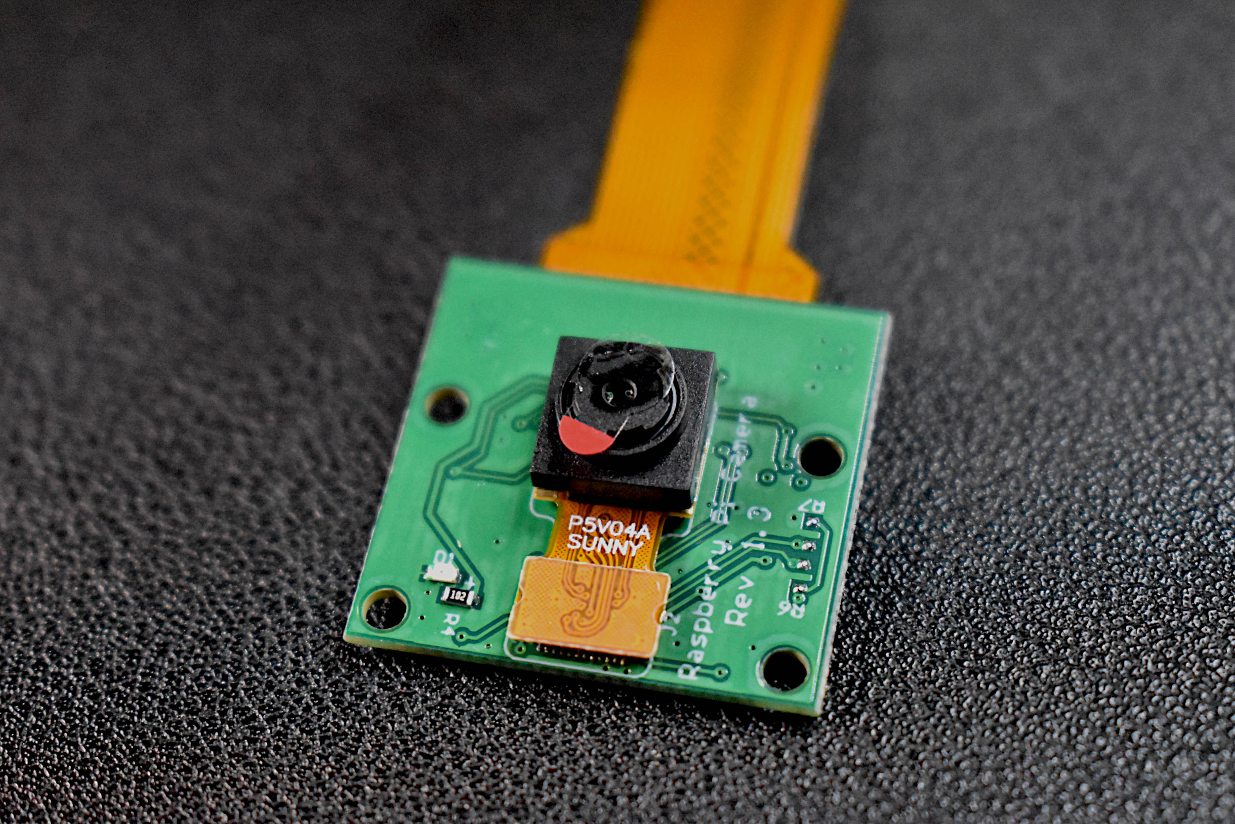
There are only two essential parts needed for this tutorial: the Raspberry Pi and the picamera. There are two picameras available, however, I will be using the older and cheaper version, V1.3, which is a 5MP camera that can record HD video. The other picamera should work just as well, the V2, which boasts 8MP, but the same video quality. I don’t imagine there are any differences in application between the two, so I will proceed under the assumption that either suffices.
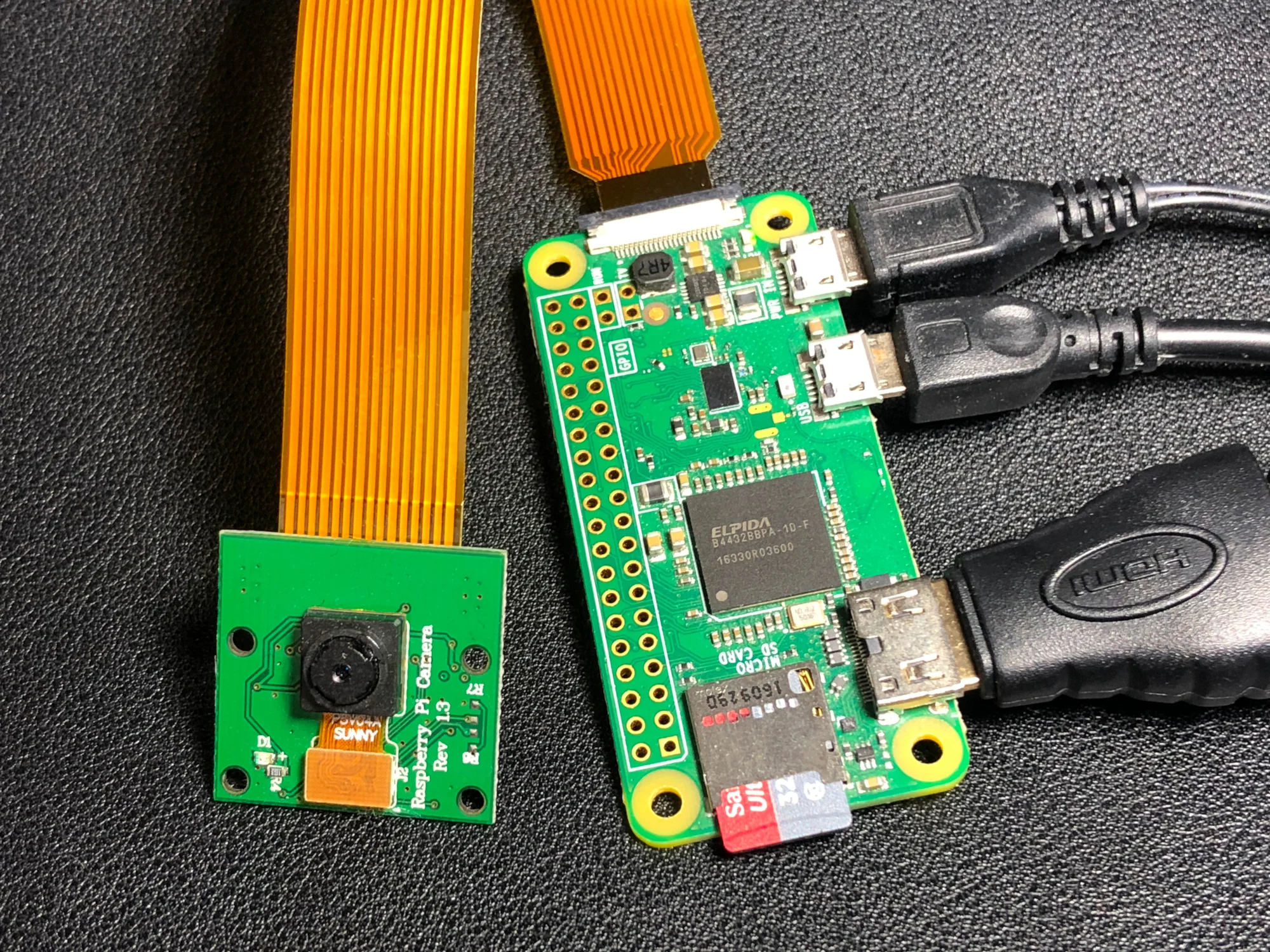
Wiring the picamera to the RPi is quite simple - both the picamera and the Pi have ribbon inputs where the thick ribbon cable is inputted. For the RPi Zero, the ribbon cable tapers to a thinner profile, which is where the Pi should be wired. The silver tracks should always be in contact with the tracks its being connected to - be wary of mistaking this, as the tracks on the ribbon can be damaged if the ribbon is inserted incorrectly into the Pi or picamera slots. If the wiring is still unclear, see the image below. Notice the black strip facing upward when wiring the ribbon to the slot. Keeping the black strip on the same side as the white casing is required for both the picamera and Pi Zero slots.

Proper Wiring of Picamera to RPi Zero W
There are numerous ‘getting started with the picamera’ tutorials out there, and so I will merely mention a few recommended tutorials and briefly explain how to prepare the picamera for use with the Pi and Python. The best ‘getting started’ tutorials are listed below:
For the absolute picamera beginner - https://projects.raspberrypi.org/en/projects/getting-started-with-picamera
Python picamera methods - https://picamera.readthedocs.io/en/release-1.13/recipes1.html
RPi + Python OpenCV Tutorial - https://www.pyimagesearch.com/2015/03/30/accessing-the-raspberry-pi-camera-with-opencv-and-python/
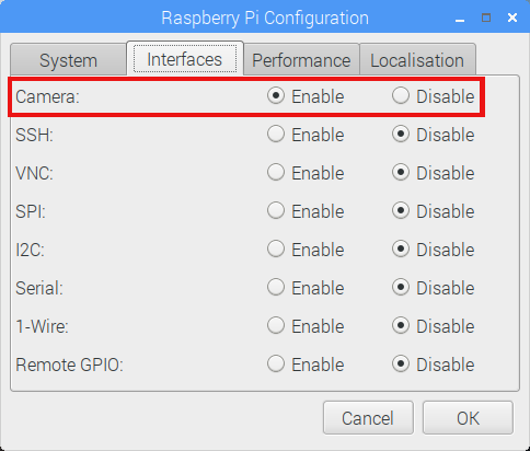
The starting point for getting the picamera working is to ensure that it is enabled in the Raspberry Pi Configuration. You can do this (most simply) by going to ‘Preferences->Raspberry Pi Configuration’ and selecting the ‘interfaces’ tab, and finally clicking ‘enable’ next to the camera option. Then click OK. The Pi may need to restart after this process. The visual steps are shown below for reference.

Once the camera module is enabled, it’s time to verify that the version of Python being used has the picamera library installed. The easiest way to do this is to open up IDLE (I’m using Python 3.5.3), and import the picamera module as shown below:
import picamera
If an error results after the import, then follow the instructions outlined in the picamera Python installation page (link here). If there was no error, we can proceed and verify that Python is communicating properly with the picamera and the camera is functioning as expected.
The code below outputs a 5 second full screen preview, takes a static image, and saves it as a .jpg file. Upon verification of the saved image, we can conclude that the picamera and Python picamera library are working together, and the image processing portion of this tutorial can begin.
from time import sleep
from picamera import PiCamera

camera = PiCamera()
camera.resolution = (2560,1936)
camera.start_preview()
sleep(5)
camera.capture('test.jpg')
camera.stop_preview()
For analysis reasons, objects of red, green, and blue were chosen to match the sub-pixel receptors of the camera (red, blue, green - RGB). I selected three breadboards, one of each color, as my test objects. The full-scale image (2560x1920 pixels) is shown below and was taken using the method given in the code above.

Raw Output (cropped) From The Raspberry Pi Camera
The quality of the photo is quite poor and this is due to the relatively low resolution of the camera (only 5MP) and the lack of processing routines available in most modern cameras. The poor quality is not important for our analysis, as much of what will be explored will involve general shapes and colors in images - something that doesn’t require sharpness or visually pleasure color palettes.
Numpy and matplotlib will be used to analyze and plot images taken by the picamera. To start, the simplest method for plotting the images is using matplotlib’s ‘imshow’ function, which plots all three RGB colors in a traditional format seen by the human eye. The code for showing an image using this method is shown below:
from picamera import PiCamera
import numpy as np
import matplotlib.pyplot as plt

h = 1024 # change this to anything < 2592 (anything over 2000 will likely get a memory error when plotting
cam_res = (int(h),int(0.75*h)) # keeping the natural 3/4 resolution of the camera
# we need to round to the nearest 16th and 32nd (requirement for picamera)
cam_res = (int(16*np.floor(cam_res[1]/16)),int(32*np.floor(cam_res[0]/32)))
# camera initialization
cam = PiCamera()
cam.resolution = (cam_res[1],cam_res[0])
data = np.empty((cam_res[0],cam_res[1],3),dtype=np.uint8) # preallocate image
while True:
    try:
        cam.capture(data,'rgb') # capture RGB image
        plt.imshow(data) # plot image
        # clear data to save memory and prevent overloading of CPU
        data = np.empty((cam_res[0],cam_res[1],3),dtype=np.uint8)
        plt.show() # show the image
        # press enter when ready to take another photo
        input("Click to save a different plot")
    # pressing CTRL+C exits the loop
    except KeyboardInterrupt:
        break
The plot should look something like the figure below, where the image’s origin is the top left corner of the plot. We will be using this as the general layout for analyzing the images taken by the picamera.

Next, we can decompose the image into its three color components: red, green, and blue. The code to do this is shown below, with an example plot showing the true color image with its three color components.
import time
from picamera import PiCamera
import numpy as np
import matplotlib.pyplot as plt

t1 = time.time()
h = 640 # change this to anything < 2592 (anything over 2000 will likely get a memory error when plotting
cam_res = (int(h),int(0.75*h)) # keeping the natural 3/4 resolution of the camera
cam_res = (int(16*np.floor(cam_res[1]/16)),int(32*np.floor(cam_res[0]/32)))
cam = PiCamera()
cam.resolution = (cam_res[1],cam_res[0])
data = np.empty((cam_res[0],cam_res[1],3),dtype=np.uint8)
x,y = np.meshgrid(np.arange(np.shape(data)[1]),np.arange(0,np.shape(data)[0]))
cam.capture(data,'rgb')
fig,axn = plt.subplots(2,2,sharex=True,sharey=True)
fig.set_size_inches(9,7)
axn[0,0].pcolormesh(x,y,data[:,:,0],cmap='gray')
axn[0,1].pcolormesh(x,y,data[:,:,1],cmap='gray')
axn[1,0].pcolormesh(x,y,data[:,:,2],cmap='gray')
axn[1,1].imshow(data,label='Full Color')
axn[0,0].title.set_text('Red')
axn[0,1].title.set_text('Green')
axn[1,0].title.set_text('Blue')
axn[1,1].title.set_text('All')
print('Time to plot all images: {0:2.1f}'.format(time.time()-t1))
data = np.empty((cam_res[0],cam_res[1],3),dtype=np.uint8)
plt.savefig('component_plot.png',dpi=150)
plt.cla()
plt.close()

As a simple introduction into image processing, it is valid to begin by analyzing color content in an image. This can be done using a multitude of statistical tools, the easiest being normally distributed mean and standard deviation. With the image above, we can take each RGB component and calculate the average and standard deviation to arrive at a characterization of color content in the photo. This will allow us to determine what colors are contained in the image and to what frequency they occur. Since we have three identical red, blue, and green objects - we would expect each object to produce a unique color signature when introduced into the frame of the camera.
First, we need consistency from the picamera, which means we need to ensure that the picamera is not changing its shutter speed or white balance. I have done this in the code below. Next, we need to establish the background information contained in the frame of the image. I do this by taking an image of the white background (no colors) and using the data as the background ‘noise’ in the image frame. This will help us identify unique changes in color introduced into the frames by the RGB breadboards. The code for all of this, plus the mean and standard deviation of the frame is given below. Using the code below, we can identify whether a red, blue, or green breadboard has been introduced into the frame.
import time
from picamera import PiCamera
import numpy as np

# picamera setup
h = 640 # change this to anything < 2592 (anything over 2000 will likely get a memory error when plotting
cam_res = (int(h),int(0.75*h)) # keeping the natural 3/4 resolution of the camera
cam_res = (int(16*np.floor(cam_res[1]/16)),int(32*np.floor(cam_res[0]/32)))
cam = PiCamera()
## making sure the picamera doesn't change white balance or exposure
## this will help create consistent images
cam.resolution = (cam_res[1],cam_res[0])
cam.framerate = 30
time.sleep(2) #let the camera settle
cam.iso = 100
cam.shutter_speed = cam.exposure_speed
cam.exposure_mode = 'off'
gain_set = cam.awb_gains
cam.awb_mode = 'off'
cam.awb_gains = gain_set
# prepping for analysis and recording background noise
# the objects should be removed while background noise is calibrated
data = np.empty((cam_res[0],cam_res[1],3),dtype=np.uint8)
noise = np.empty((cam_res[0],cam_res[1],3),dtype=np.uint8)
x,y = np.meshgrid(np.arange(np.shape(data)[1]),np.arange(0,np.shape(data)[0]))
rgb_text = ['Red','Green','Blue'] # array for naming color
input("press enter to capture background noise (remove colors)")
cam.capture(noise,'rgb')
noise = noise-np.mean(noise) # background 'noise'
# looping with different images to determine instantaneous colors
while True:
    try:
        print('===========================')
        input("press enter to capture image")
        cam.capture(data,'rgb')
        mean_array,std_array = [],[]
        for ii in range(0,3):
            # calculate mean and STDev and print out for each color
            mean_array.append(np.mean(data[:,:,ii]-np.mean(data)-np.mean(noise[:,:,ii])))
            std_array.append(np.std(data[:,:,ii]-np.mean(data)-np.mean(noise[:,:,ii])))
            print('-------------------------')
            print(rgb_text[ii]+'---mean: {0:2.1f}, stdev: {1:2.1f}'.format(mean_array[ii],std_array[ii]))
        # guess the color of the object
        print('--------------------------')
        print('The Object is: {}'.format(rgb_text[np.argmax(mean_array)]))
        print('--------------------------')
    except KeyboardInterrupt:
        break
The code should print out the mean and standard deviation of each color component, and also predict the color of the object inserted into the frame. A sample printout is shown below:
===========================
press enter to capture image
-------------------------
Red---mean: -2.2, stdev: 30.6
-------------------------
Green---mean: 1.2, stdev: 23.8
-------------------------
Blue---mean: 1.0, stdev: 24.8
--------------------------
The Object is: Green
--------------------------
The user may notice that complications arise when multiple colors are present in the image. This is because the background information has drastically changed with the introduction of multiple colors. This results in uneven statistical relevance in the reading of each color when compared to the background noise. Therefore, for multiple object color recognition, more complex spatial tools are needed to identify regions of colors. This is a complication that will be reserved for the next entry into the image processing series.
A video demonstration of this is given below:
In the first entry into the Image Processing Using Raspberry Pi and Python, the picamera and its Python library were introduced as basic tools for real-time analysis. Additionally, simple tools for plotting an image and its components were explored, along with more complex tools involving statistical distributions of colors. The combination of picamera and Python is a powerful tool with applications where differentiating colors may be of importance. One application comes to mind involving industrial quality control, where color consistency may be of utmost importance. Moreover, the ability to analyze images in real-time is a tool that exists in many technologies ranging from smartphone facial recognition, to security systems, and even autonomous vehicle navigation. For the next entry in the Image Processing tutorial series, spatial identification tools will be explored with applications in object detection and color classification.


See More in Raspberry Pi and Engineering: